9 The Theoretical Model

Objectives of this page

This page presents the DSGE model from the paper and two simplified versions (an RBC model and a New Keynesian model).

The model in the paper is built in an RBC framework (no nominal effects+rational expectations). It is designed for a small open economy (home vs. world). There are two sectors in it: a weather-dependent agricultural sector, and a standard non-agricultural sector. It is assumed that weather shocks affect the agricultural sector through a damage function.

9.1 Model Used in the Paper

9.1.1 Overview of the Model

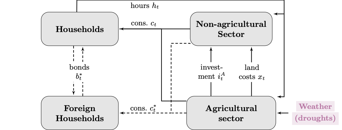
Our model is a two-sector, two-good economy in a small open economy setup with a flexible exchange rate regime. The home economy is populated by households and firms. The latter operate in the agricultural and the non-agricultural sectors. Workers from the agricultural sector face unexpected weather conditions that affect the productivity of their land. Households consume both home and foreign varieties of goods, thus creating a trading channel adjusted by the real exchange rate. The general structure of the model is summarized in Figure 9.1.

Important

Please refer to the paper for a full description of the model.

In this notebook, we only remind the main specificities of the model.

9.1.2 Agricultural sector and the weather

We assume the weather follows an univariate stochastic exogenous process: \[ \log(\colorbox{wongPurple!17}{\textbf{\textcolor{wongPurple}{$\varepsilon_{t}^{W}$}}})=\rho_{W}\log(\colorbox{wongPurple!17}{\textbf{\textcolor{wongPurple}{$\varepsilon_{t-1}^{W}$}}})+\sigma_{W}\eta_{t}^{W},\text{\ \ \ \ \ }\eta_{t}^{W}\sim\mathcal{N}\left( 0,1\right) \tag{9.1}\]

where $\color{wongPurple}\varepsilon_{t}^{W}>1$ features a drought.

Each farmer $i\in\left[ n,1\right]$ has a land endowment $\color{wongGreen}\ell_{it}$ whose time-varying productivity (or efficiency) writes: \[ {\color{wongGreen}\ell_{it}}=\left( 1-\delta_{\ell}\right) {\color{wongOrange}\Omega\left( \varepsilon_{t}^{W}\right)} {\color{wongGreen}\ell_{it-1}} + x_{it}, \tag{9.2}\]

where $\delta_{\ell}\in(0,1)$ is the rate of decay of land efficiency, $x_{it}$ are intermediate goods to maintain land efficiency (crops, water, fertilizers…), $\color{wongOrange}\Omega\left( \varepsilon_{t}^{W}\right)$ is a weather damage function. We opt for a simple functional form for this weather damage function: \[ {\color{wongOrange}\Omega\left( \varepsilon_{t}^{W}\right)} =\left( {\color{wongPurple}\varepsilon_{t}^{W}}\right)^{-{\color{wongLightBlue}\theta}}, \tag{9.3}\]

where $\color{wongLightBlue}\theta$ is the elasticity of land productivity with respect to the weather variations.

Following IAMs models pioneered by Nordhaus (1991), the damage function bridges the weather with economic conditions. To avoid concerns from Pindyck (2017) :

Our setup is linear (i.e., we don’t exploit the non-linearity of the damage function).
$\color{wongLightBlue}\theta$ is estimated agnostically (through a very diffuse prior).

The profits of the farmer write: \[ {\color{wongBlue}d_{it}^{A}}=p_{t}^{A}y_{it}^{A}-p_{t}^{N}\left( i_{it}^{A}+S\left(\varepsilon_{t}^{i}\frac{i_{it}^{A}}{i_{it-1}^{A}}\right) i_{it-1}^{A}\right)-w_{t}^{A}h_{it}^{A}-p_{t}^{N}{\color{wongGreen}v\left( x_{it}\right)}, \tag{9.4}\]

For the land cost function $\color{gris}v\left( x_{it}\right)$, we opt for an unopiniated form: \[ {\color{gris}v\left( x_{it}\right)} =\frac{\tau}{1+{\color{wongOrange}\phi}}x_{it}^{1+{\color{wongOrange}\phi}} \tag{9.5}\]

where $\tau>0$ is a scale parameter; $\color{wongOrange}\phi$ is the elasticity of intermediate input to land:

$\color{wongOrange}\phi>0$ land costs exhibits increasing returns, $\color{wongOrange}\phi=0$ linear returns and $\color{wongOrange}\phi<0$ decreasing returns.
Data favors $\color{wongOrange}\phi\geq0$ (as weather shocks generate recessions).

Lastly, the optimization of profits is given by: \[ \begin{align*} & \max_{\left\{ h_{it}^{A},i_{it}^{A},k_{it}^{A},\ell_{it}\right\} }% E_{t}\sum\limits_{\tau=0}^{\infty}\left\{ \Lambda_{t,t+\tau}{\color{wongLightBlue}d_{it+\tau}^{A}}\right\} \\ \text{s.t. } y_{it}^{A} & =\varepsilon_{t}^{Z}{\color{wongGreen}\ell_{it-1}^{\omega}}\left[ \left( k_{it-1}^{A}\right) ^{\alpha}\left( \kappa_{A}h_{it}^{A}\right)^{1-\alpha}\right] ^{1-\omega}\\ \text{s.t. }i_{it}^{A} &= k_{it}^{A}-\left( 1-\delta_{K}\right) k_{it-1}^{A} \end{align*} \] First Order Conditions on land $\color{wongGreen}\ell_{it}$:

$\underset{\text{current marginal land cost}}{\underbrace{\underset{}{p_{t}^{N}}{\color{gris}v^{\prime}\left( x_{it}\right)}}} = \underset{\text{expected marginal gains}}{\underbrace{E_{t}\left\{\Lambda_{t,t+1}\left[\omega p_{t+1}^{A}\frac{y_{it+1}^{N}}{\ell_{it}}+\left(1-\delta_{\ell}\right){\color{wongOrange}\Omega\left( \varepsilon_{t+1}^{W}\right)} p_{t+1}^{N}{\color{gris}v^{\prime}\left(x_{it+1}\right)}\right]\right\} }}$

9.2 Simplified Two-Sector Weather RBC Model

9.2.1 Households

A representative household consumes a CES bundle of agricultural and non-agricultural goods. Consumption with habits is defined as \[ \tilde c_t = c_t - b c_{t-1}. \tag{9.6}\]

Preferences are \[ U = \mathbb{E}_0 \sum_{t=0}^{\infty} \beta^t \left[ \frac{\tilde c_t^{\,1-\sigma_C}}{1-\sigma_C} - \chi\, h_{u,t}^{\,1+\sigma_H} \right], \tag{9.7}\] where the labor aggregator, capturing reallocation costs, is \[ h_{u,t} = \left(h_{N,t}^{1+\iota} + h_{A,t}^{1+\iota}\right)^{\frac{1}{1+\iota}}. \tag{9.8}\]

The marginal utility of consumption and the stochastic discount factor are \[ u_{c,t} = \tilde c_t^{-\sigma_C}, \qquad m_t = \beta \frac{u_{c,t}}{u_{c,t-1}}. \tag{9.9}\]

Intratemporal optimality conditions: \[ w^N_t\, u_{c,t} = u^N_t, \qquad w^A_t\, u_{c,t} = u^A_t, \tag{9.10}\] with \[ u^N_t = e^h_t\, \chi\, h_{u,t}^{\sigma_H}\left(\frac{h_{N,t}}{h_{u,t}}\right)^\iota, \qquad u^A_t = e^h_t\, \chi\, h_{u,t}^{\sigma_H}\left(\frac{h_{A,t}}{h_{u,t}}\right)^\iota. \tag{9.11}\]

Euler equation: \[ m_{t+1} r_{t+1} = 1. \tag{9.12}\]

9.2.2 Production

There are two sectors: non-agriculture and agriculture.

Non-agricultural production:

\[ y^N_t = e^z_t\, h_{N,t}^{\,1-\alpha}. \tag{9.13}\]

Optimal labor demand: \[ w^N_t = (1-\alpha)\, p^N_t \frac{y^N_t}{h_{N,t}}. \tag{9.14}\]

Agricultural output is \[ y^A_t = (d_t\,\ell_{t-1})^{\omega} \left(e^z_t \kappa_A\, h_{A,t}^{\,1-\alpha}\right)^{1-\omega}, \tag{9.15}\] where the weather damage factor is \[ d_t = (e^s_t)^{-\theta_1}. \tag{9.16}\]

Labor demand: \[ w^A_t = (1-\omega)(1-\alpha)\, p^A_t\,\frac{y^A_t}{h_{A,t}}. \tag{9.17}\]

Land evolves according to \[ \ell_t = (1-\delta_L)\,d_t\, \ell_{t-1} + \phi_t, \tag{9.18}\] where $\phi_t$ is land investment.

Land cost function: \[ \phi_t = \frac{\tau}{\psi}\, x_t^{\psi}\, d_t\, \ell_{t-1}. \tag{9.19}\]

Shadow value of land $\varrho_t$ satisfies \[ \varrho_t = m_{t+1} \left[ \frac{\omega\, p^A_{t+1} y^A_{t+1}}{\ell_t} + (1-\delta_L)d_{t+1}\varrho_{t+1} + \frac{\phi_{t+1}}{\ell_t} \right]. \tag{9.20}\]

FOC for land investment $x_t$: \[ p^N_t = \tau\, x_t^{\psi-1}\, \varrho_t\, d_t\, \ell_{t-1}. \tag{9.21}\]

9.2.3 Aggregation and Prices

Let $n_t$ be the agricultural sector share: \[ n_t = \bar n\, e^n_t. \tag{9.22}\]

Aggregate output: \[ y_t = (1-n_t)\, p^N_t y^N_t + n_t\, p^A_t y^A_t. \tag{9.23}\]

Aggregate hours: \[ h_t = (1-n_t) h_{N,t} + n_t h_{A,t}. \tag{9.24}\]

Consumption demand across sectors, with non-agricultural goods: \[ (1-n_t) y^N_t = (1-\varphi)\, (p^N_t)^{-\mu}\, c_t + n_t x_t + g_y\, \bar y^N\, e^g_t. \tag{9.25}\]

and agricultural goods: \[ n_t y^A_t = \varphi\, (p^A_t)^{-\mu}\, c_t. \tag{9.26}\]

Relative price index:

\[ 1 = (1-\varphi) (p^N_t)^{1-\mu} + \varphi (p^A_t)^{1-\mu}. \tag{9.27}\]

Gross Domestic Product:

\[ GDP_t = y_t - n_t p^N_t x_t. \tag{9.28}\]

Shock processes:

All shocks follow AR(1) laws of motion: \[ \log e^z_t = \rho_z \log e^z_{t-1} + \sigma_z\, \eta^z_t, \tag{9.29}\] \[ \log e^h_t = \rho_h \log e^h_{t-1} + \sigma_h\, \eta^h_t, \tag{9.30}\] \[ \log e^g_t = \rho_g \log e^g_{t-1} + \sigma_g\, \eta^g_t, \tag{9.31}\] \[ \log e^n_t = \rho_n \log e^n_{t-1} + \sigma_n\, \eta^n_t, \tag{9.32}\] \[ \log e^s_t = \rho_s \log e^s_{t-1} + \sigma_s\, \eta^s_t. \tag{9.33}\]

All innovations $\eta^j_t$ are i.i.d. standard normal.

9.3 Two Sector New Keynesian Model with Weather Shocks and Land

9.3.1 Households

A representative household consumes a CES bundle of agricultural and non agricultural goods and supplies differentiated labor to the two sectors.

Habit adjusted consumption: \[ \tilde c_t = c_t - b c_{t-1}. \tag{9.34}\]

Preferences: \[ U = \mathbb{E}_0 \sum_{t=0}^{\infty} \beta^t \left[ \frac{\tilde c_t^{\,1-\sigma_C}}{1-\sigma_C} - \chi\, h_{u,t}^{\,1+\sigma_H} \right], \tag{9.35}\] where the labor aggregator with reallocation costs is \[ h_{u,t} = \left(h_{N,t}^{1+\\iota} + h_{A,t}^{1+\\iota}\right)^{\frac{1}{1+\\iota}}. \tag{9.36}\]

Marginal utility of consumption and stochastic discount factor: \[ u_{c,t} = \tilde c_t^{-\sigma_C}, \qquad m_t = \beta \frac{u_{c,t}}{u_{c,t-1}}. \tag{9.37}\]

Intratemporal optimality: \[ w^N_t\, u_{c,t} = u^N_t, \qquad w^A_t\, u_{c,t} = u^A_t, \tag{9.38}\] with sector specific marginal disutilities of labor \[ u^N_t = e^h_t\, \chi\, h_{u,t}^{\sigma_H}\left(\frac{h_{N,t}}{h_{u,t}}\right)^\iota, \qquad u^A_t = e^h_t\, \chi\, h_{u,t}^{\sigma_H}\left(\frac{h_{A,t}}{h_{u,t}}\right)^\iota. \tag{9.39}\]

Nominal Euler equation (one period nominal bond): \[ m_{t+1} \frac{R_t}{\pi_{t+1}} = 1, \tag{9.40}\] where $R_t$ is the gross nominal interest rate and $\pi_t$ is gross aggregate inflation.

9.3.2 Production

The economy has two producing sectors: non agriculture ($N$) and agriculture ($A$).

9.3.2.1 Non-Agricultural Sector

Production is linear in TFP and concave in labor: \[ y^N_t = e^z_t\, h_{N,t}^{\,1-\alpha}. \tag{9.41}\]

With real marginal cost $mc^N_t$, cost minimization implies: \[ w^N_t = mc^N_t (1-\alpha)\, p^N_t \frac{y^N_t}{h_{N,t}}, \tag{9.42}\] where $p^N_t$ is the relative price of non agricultural goods.

9.3.2.2 Agricultural sector with land and weather damage.

Weather affects agricultural production through a damage function. Let $d_t$ denote the weather damage factor \[ d_t = (e^s_t)^{-\theta_1}. \tag{9.43}\]

Agricultural output: \[ y^A_t = (d_t\,\ell_{t-1})^{\omega} \left(e^z_t \kappa_A\, h_{A,t}^{\,1-\alpha}\right)^{1-\omega}. \tag{9.44}\]

With real marginal cost $mc^A_t$, labor demand in agriculture: \[ w^A_t = mc^A_t (1-\omega)(1-\alpha)\, p^A_t\,\frac{y^A_t}{h_{A,t}}, \tag{9.45}\] where $p^A_t$ is the relative price of agricultural goods.

9.3.3 Price setting and nominal rigidities

Prices are sticky in both sectors. We adopt Rotemberg type quadratic adjustment costs on inflation. For sector $j \in \{N,A\}$, let $\epsilon_j$ denote the elasticity of substitution and $\kappa_j$ the adjustment cost parameter.

Denote sectoral inflation by $\pi_{j,t}$ and aggregate inflation by $\pi_t$. The New Keynesian Phillips curves in each sector take the form \[ (1-\epsilon_j)\, p^j_t y^j_t + \epsilon_j\, mc^j_t y^j_t - \kappa_j\, p^j_t \pi_{j,t}(\pi_{j,t}-1)\, y^j_t + \kappa_j\, \mathbb{E}_t\left[ m_{t+1} p^j_{t+1} \pi_{j,t+1}(\pi_{j,t+1}-1)\, y^j_{t+1} \right] = 0, \tag{9.46}\] for $j = N,A$.

9.3.4 Land, land costs, and damage

Land evolves according to \[ \ell_t = (1-\delta_L)\,d_t\, \ell_{t-1} + \phi_t, \tag{9.47}\] where $\phi_t$ is land investment.

Land cost function: \[ \phi_t = \frac{\tau}{\psi}\, x_t^{\psi}\, d_t\, \ell_{t-1}, \tag{9.48}\] with $x_t$ the land investment intensity.

Shadow value of land $\varrho_t$ satisfies \[ \varrho_t = \mathbb{E}_t\left\{ m_{t+1} \left[ mc^A_{t+1}\frac{\omega\, p^A_{t+1} y^A_{t+1}}{\ell_t} + (1-\delta_L)d_{t+1}\varrho_{t+1} + \frac{\phi_{t+1}}{\ell_t} \right] \right\}. \tag{9.49}\]

FOC for land investment $x_t$: \[ p^N_t = \tau\, x_t^{\psi-1}\, \varrho_t\, d_t\, \ell_{t-1}. \tag{9.50}\]

9.3.5 Aggregation, demand, and prices

Let $n_t$ be the agricultural sector share, driven by a reallocation shock: \[ n_t = \bar n\, e^n_t. \tag{9.51}\]

Aggregate output: \[ y_t = (1-n_t)\, p^N_t y^N_t + n_t\, p^A_t y^A_t. \tag{9.52}\]

Aggregate hours: \[ h_t = (1-n_t) h_{N,t} + n_t h_{A,t}. \tag{9.53}\]

Non agricultural goods: \[ (1-n_t) y^N_t = (1-\varphi)\, (p^N_t)^{-\mu}\, c_t + n_t x_t + g_y\, \bar y^N\, e^g_t. \tag{9.54}\]

Agricultural goods: \[ n_t y^A_t = \varphi\, (p^A_t)^{-\mu}\, c_t. \tag{9.55}\]

9.3.5.1 Relative price index

The CES price index is \[ 1 = (1-\varphi) (p^N_t)^{1-\mu} + \varphi (p^A_t)^{1-\mu}. \tag{9.56}\]

Inflation measures, let $P_t$ denote the aggregate price index. Gross inflation is \[ \pi_t = \frac{P_t}{P_{t-1}}. \tag{9.57}\] Sectoral inflation rates are \[ \pi_{N,t} = \frac{P^N_t}{P^N_{t-1}}, \qquad \pi_{A,t} = \frac{P^A_t}{P^A_{t-1}}. \tag{9.58}\]

Gross Domestic Product:

\[ GDP_t = y_t - n_t p^N_t x_t. \tag{9.59}\]

9.3.6 Monetary policy

Monetary policy follows a Taylor rule in logs around the steady state: \[ \log\left(\frac{R_t}{\bar R}\right) = \rho\, \log\left(\frac{R_{t-1}}{\bar R}\right) + (1-\rho)\left[ \phi_y \log\left(\frac{GDP_t}{\overline{GDP}}\right) + \phi_\pi \log(\pi_t) \right], \tag{9.60}\] where $\bar R$ and $\overline{GDP}$ denote steady state values.

9.3.7 Shock processes

All exogenous processes follow AR(1) dynamics: \[ \log e^z_t = \rho_z \log e^z_{t-1} + \sigma_z\, \eta^z_t, \tag{9.61}\] \[ \log e^h_t = \rho_h \log e^h_{t-1} + \sigma_h\, \eta^h_t, \tag{9.62}\] \[ \log e^g_t = \rho_g \log e^g_{t-1} + \sigma_g\, \eta^g_t, \tag{9.63}\] \[ \log e^n_t = \rho_n \log e^n_{t-1} + \sigma_n\, \eta^n_t, \tag{9.64}\] \[ \log e^s_t = \rho_s \log e^s_{t-1} + \sigma_s\, \eta^s_t. \tag{9.65}\]

All innovations $\eta^j_t$ are iid standard normal.