4 Weather Data: Missing Data

Objectives of this page

This chapter examines and imputes missing observations in the gridded weather data from Chapter 3.

library(tidyverse)

── Attaching core tidyverse packages ──────────────────────── tidyverse 2.0.0 ──
✔ dplyr     1.1.4     ✔ readr     2.1.5
✔ forcats   1.0.0     ✔ stringr   1.5.2
✔ ggplot2   4.0.0     ✔ tibble    3.3.0
✔ lubridate 1.9.4     ✔ tidyr     1.3.1
✔ purrr     1.1.0     
── Conflicts ────────────────────────────────────────── tidyverse_conflicts() ──
✖ dplyr::filter() masks stats::filter()
✖ dplyr::lag()    masks stats::lag()
ℹ Use the conflicted package (<http://conflicted.r-lib.org/>) to force all conflicts to become errors

library(sf)

Linking to GEOS 3.13.0, GDAL 3.8.5, PROJ 9.5.1; sf_use_s2() is TRUE

Let us load the graphs theme functions (See Chapter 1):

source("../scripts/functions/utils.R")

Let us also load the maps for the countries of interest (See Chapter 2).

load("../data/Maps/GADM-4.1/maps_level_0.RData")
maps_level_0_NZ <- st_shift_longitude(maps_level_0$NZL)

We focus on the countries defined in Chapter 2:

load("../output/tb_countries.rda")
tb_countries

# A tibble: 1 × 4
  country_code country_name country_name_short country_name_clear
  <chr>        <chr>        <chr>              <chr>             
1 NZL          New Zealand  New Zealand        New-Zealand

4.1 Import Data

We define a function, load_daily(), which loads the daily data obtained in Chapter 3.

#' Loads a weather data from country x year
#'
#' @param file path to the file to load
load_daily <- function(file) {
  load(file)
  weather_grid_country
}

Let us focus on New Zealand.

country <- "New Zealand"

We extract the corresponding country code:

country_code <- tb_countries |>
  dplyr::filter(country_name == !!country) |>
  dplyr::pull("country_code")

We list the files that contain the daily data for the current country:

N <- list(
  precip = "../Data/Weather/CPC/grid_daily_precip/",
  tmin = "../Data/Weather/CPC/grid_daily_tmin/",
  tmax = "../Data/Weather/CPC/grid_daily_tmax/"
) |>
  map(~list.files(.x, full.names = TRUE, pattern = str_c(country_code, "_")))

Let us load these files:

# Load precip, tmin and tmax
country_precip_daily <- map(N$precip, load_daily) |>list_rbind()
country_tmin_daily <- map(N$tmin, load_daily) |>list_rbind()
country_tmax_daily <- map(N$tmax, load_daily) |>list_rbind()

Let us merge these datasets:

country_weather_daily <- country_precip_daily |>
    dplyr::mutate(variable = "precip") |>
    bind_rows(
      country_tmin_daily  |> mutate(variable = "tmin")
    ) |>
    bind_rows(
      country_tmax_daily  |> mutate(variable = "tmax")
    ) |>
    dplyr::select(-grid_id) |>
  pivot_wider(values_from = value, names_from = variable) |> 
  group_by(longitude, latitude) |> 
  dplyr::mutate(cell_id = cur_group_id()) |> 
  ungroup()

We extract information about longitude / latitude and geometry of each cell:

cells <- country_weather_daily |> 
  dplyr::select(cell_id, longitude, latitude, geometry, intersect_area) |> 
  unique()

cells <- cells |> dplyr::mutate(country = !!country)

Let us transform this object as an sf object:

cells_sf <- st_as_sf(cells)

We can have a look at the number of values per cell.

# This code is not evaluated here.
#| code-fold: true
ggplot() + 
  geom_sf(
    data = st_as_sf(cells) |> 
      left_join(
        country_weather_daily |> group_by(cell_id) |> count() |> 
          arrange(n),
        by = "cell_id"
      ),
    mapping = aes(fill = n)
  ) +
  geom_sf(
    data = maps_level_0_NZ$NGA,
    fill = NA, col = "black"
  )

We can identify the cells for which the number of records is lower than the max number of records:

cells_to_remove <- 
  country_weather_daily |> group_by(cell_id) |> count() |> 
  ungroup() |> 
  mutate(max = max(n)) |> 
  filter(n < max)

# This code is not evaluated here.
#| code-fold: true
ggplot() + 
  geom_sf(
    data = st_as_sf(cells) |> 
      left_join(
        country_weather_daily |> group_by(cell_id) |> count() |> 
          arrange(n),
        by = "cell_id"
      ) |> 
      left_join(
        cells_to_remove |> select(cell_id) |> 
          mutate(to_remove = TRUE)
      ) |> 
      mutate(to_remove = replace_na(to_remove, FALSE)),
    mapping = aes(fill = to_remove)
  ) +
  geom_sf(
    data = maps_level_0_NZ,
    fill = NA, col = "black"
  ) +
  scale_fill_manual(
    "Remove", 
    values = c(`TRUE` = "red", `FALSE` = NA)
  )

Let us remove those cells:

country_weather_daily <- 
  country_weather_daily |> 
  filter(! cell_id %in% cells_to_remove$cell_id)

We also remove the cells corresponding to islands for which we will have no agricultural records.

ids_islands <- c(
  1, 2, 5, 6, 24, 25, 34, 35, 45, 46, 55, 56, 256, 250, 249, 255,
  264, 267, 263, 266, 261, 260, 259, 262, 265
)
country_weather_daily <- 
  country_weather_daily |> 
  filter(
    ! cell_id %in% ids_islands
  )

Code

# This chunk is not evaluated here.
ggplot() + 
  geom_sf(
    data = st_as_sf(cells) |> 
      inner_join(
        country_weather_daily |> group_by(cell_id) |> count() |> 
          arrange(n),
        by = "cell_id"
      ),
    fill = "red"
  ) +
  geom_sf(
    data = maps_level_0_NZ,
    fill = NA, col = "black"
  )

cells <- 
  cells |> filter(
  ! cell_id %in% c(cells_to_remove$cell_id, ids_islands)
)

cells_sf <- st_as_sf(cells)

Let us save this grid:

save(
  cells,
  file = str_c("../data/Weather/CPC/", country_code, "_cells.RData")
)

We remove the geometry from the table:

country_weather_daily <- 
  country_weather_daily |> 
  dplyr::select(-geometry, -intersect_area)

The total number of observations:

scales::number(nrow(country_weather_daily), big.mark = ",")

[1] "2,975,097"

4.2 Missing Values

How many missing values are there here in the dataset?

country_weather_daily |> 
  summarise(across(everything(), ~sum(is.na(.x))))

# A tibble: 1 × 8
  longitude latitude country_code  date precip   tmin   tmax cell_id
      <int>    <int>        <int> <int>  <int>  <int>  <int>   <int>
1         0        0            0     0  16895 446893 445241       0

4.2.1 Precipitation

The number of missing data for precipitation per cell:

tb_nb_na_precip <- country_weather_daily |> 
  group_by(cell_id) |> 
  select(cell_id, precip) |> 
  summarise(nb_na_precip = sum(is.na(precip))) |> 
  arrange(desc(nb_na_precip))
tb_nb_na_precip

# A tibble: 181 × 2
   cell_id nb_na_precip
     <int>        <int>
 1     153         9875
 2       9           39
 3      12           39
 4      13           39
 5      14           39
 6      19           39
 7      20           39
 8      21           39
 9      22           39
10      27           39
# ℹ 171 more rows

What if we look at missing values per cell and day?

country_weather_daily |> 
  group_by(date) |> 
  summarise(nb_na_precip = sum(is.na(precip))) |> 
  filter(nb_na_precip > 0) |> 
  arrange(desc(nb_na_precip)) |> 
  DT::datatable()

And by cell?

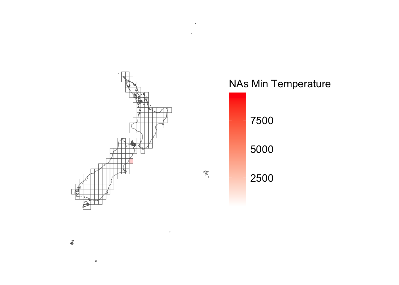
ggplot() +
  geom_sf(
    data = cells_sf |> 
      left_join(tb_nb_na_precip),
    alpha = .2,
    mapping = aes(fill = nb_na_precip)
  ) +
  geom_sf(data = maps_level_0_NZ, fill = NA) +
  scale_fill_gradient("NAs Min Temperature", low = "white", high = "red") +
  theme_map_paper()

Joining with `by = join_by(cell_id)`

Figure 4.1: Number of missing values for precipitation per cell

Most missing precipitation observations are from cell 153 which is covering a tiny fraction of land.

4.2.2 Minimum Temperatures

Now, let us do the same for min temperatures:

tb_nb_na_tmin <- country_weather_daily |> 
  group_by(cell_id) |> 
  select(cell_id, tmin) |> 
  summarise(nb_na_tmin = sum(is.na(tmin))) |> 
  arrange(desc(nb_na_tmin))
tb_nb_na_tmin

# A tibble: 181 × 2
   cell_id nb_na_tmin
     <int>      <int>
 1     152      16437
 2     171      16437
 3     196      16437
 4     221      16437
 5     239      16437
 6     258      16437
 7       9       6979
 8      14       6979
 9      22       6979
10      27       6979
# ℹ 171 more rows

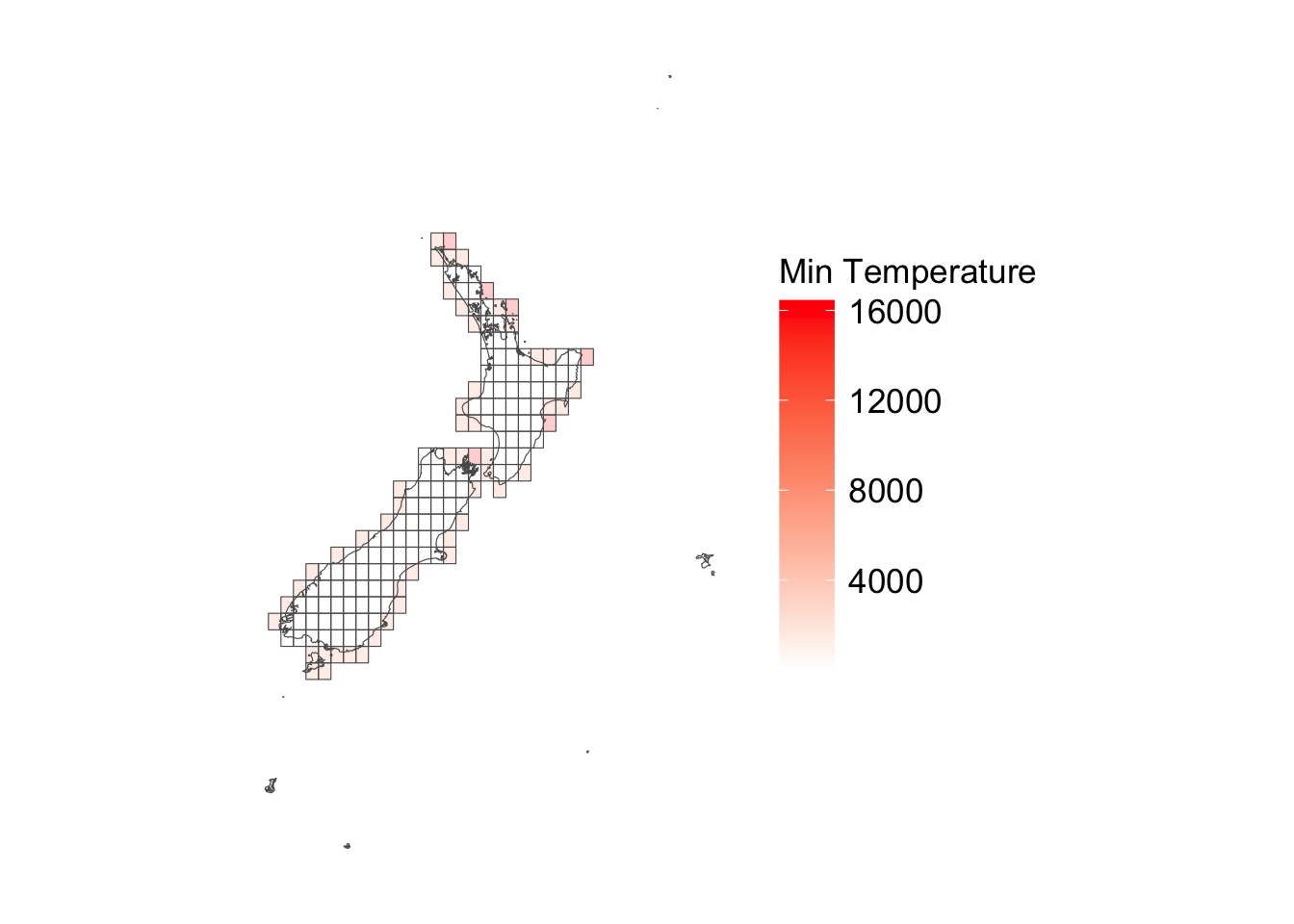
ggplot() +
  geom_sf(
    data = cells_sf |> 
      left_join(tb_nb_na_tmin),
    alpha = .2,
    mapping = aes(fill = nb_na_tmin)
  ) +
  geom_sf(data = maps_level_0_NZ, fill = NA) +
  scale_fill_gradient("Min Temperature", low = "white", high = "red") +
  theme_map_paper()

Joining with `by = join_by(cell_id)`

Figure 4.2: Number of missing values for minimum temperatures per cell

Spatially, missing observation are mostly on coastal areas.

For each cell, the number of daily observations from 1980-01-01 to 2024-12-31 is:

seq(
  min(country_weather_daily$date), 
  max(country_weather_daily$date), 
  by = "day"
) |> 
  length()

[1] 16437

What if we look at missing values per cell and day?

country_weather_daily |> 
  group_by(date) |> 
  summarise(nb_na_tmin = sum(is.na(tmin))) |> 
  filter(nb_na_tmin > 10) |> 
  arrange(desc(nb_na_tmin)) |> 
  DT::datatable()

4.2.3 Maximum Temperatures

And for max temperatures:

tb_nb_na_tmax <- 
  country_weather_daily |> 
  group_by(cell_id) |> 
  select(cell_id, tmax) |> 
  summarise(nb_na_tmax = sum(is.na(tmax))) |> 
  arrange(desc(nb_na_tmax))
tb_nb_na_tmax

# A tibble: 181 × 2
   cell_id nb_na_tmax
     <int>      <int>
 1     152      16437
 2     171      16437
 3     196      16437
 4     221      16437
 5     239      16437
 6     258      16437
 7       9       6971
 8      14       6971
 9      22       6971
10      27       6971
# ℹ 171 more rows

ggplot() +
  geom_sf(
    data = cells_sf |> 
      left_join(tb_nb_na_tmax),
    alpha = .2,
    mapping = aes(fill = nb_na_tmax)
  ) +
  geom_sf(data = maps_level_0_NZ, fill = NA) +
  scale_fill_gradient("Max Temperature", low = "white", high = "red") +
  theme_map_paper()

Joining with `by = join_by(cell_id)`

Figure 4.3: Number of missing values for maximum temperatures per cell

What if we look at missing values per cell and day?

country_weather_daily |> 
  group_by(date) |> 
  summarise(nb_na_tmax = sum(is.na(tmax))) |> 
  filter(nb_na_tmax > 10) |> 
  arrange(desc(nb_na_tmax)) |> 
  DT::datatable()

4.3 Temporal Interpolation

Let us use splines at the cell level to interpolate missing values for which no more than 5 consecutive values are missing. We will then address the interpolation of missing values for the south-western cells.

country_weather_daily <- 
  country_weather_daily |> 
  arrange(date) |> 
  nest(.by = cell_id) |> 
  mutate(
    precip_new = map(data, ~{
      if (sum(is.na(.x$precip)) >= nrow(.x)-1) {
        new_val <- NA
      } else {
        new_val <- imputeTS::na_interpolation(.x$precip, maxgap = 5, option = "spline")
      }
      new_val}
    ),
    tmin_new = map(data, ~{
      if (sum(is.na(.x$tmin)) >= nrow(.x)-1) {
        new_val <- NA
      } else {
        new_val <- imputeTS::na_interpolation(.x$tmin, maxgap = 5, option = "spline")
      }
      new_val}
    ),
    tmax_new = map(data, ~{
      if (sum(is.na(.x$tmax)) >= nrow(.x)-1) {
        new_val <- NA
      } else {
        new_val <- imputeTS::na_interpolation(.x$tmax, maxgap = 5, option = "spline")
      }
      new_val}
    )
  ) |> 
  unnest(cols = c(data, precip_new, tmin_new, tmax_new))

Registered S3 method overwritten by 'quantmod':
  method            from
  as.zoo.data.frame zoo

With the interpolation, there might be negative values, which is not possible for precipitation. We set to 0 precipitation for which interpolated values are negative.

country_weather_daily <- 
  country_weather_daily |> 
  mutate(
    precip_new = ifelse(precip_new < 0, 0, precip_new)
  )

4.4 Spatial Interpolation

Now, let us address the problem of the remaining cells for which we have some missing observation. First, we identify cells IDs for which observations are missing for precipitation, and for min and max temperatures.

cell_id_missing_precip <- 
  tb_nb_na_precip |> pull(cell_id)
cell_id_missing_tmin <- 
  tb_nb_na_tmin |> pull(cell_id)
cell_id_missing_tmax <- 
  tb_nb_na_tmax |> pull(cell_id)

We will replace the missing observations with weighted averages of the values found in the neighbors cells. We will consider the 5 nearest cells and use the inverse distance to those as the weights in the weighted average.

First, let us get the distance matrix of the cells, using the centroid of each cell as the reference point.

centroids_cells <- sf::st_centroid(cells_sf)

Warning: st_centroid assumes attributes are constant over geometries

distance_matrix <- sf::st_distance(centroids_cells, centroids_cells)

We can then define the find_neighbors_radius() function which returns the cells within a radius of another cell:

#' Identifies the neighbors of a cell given a radius
#' @param id cell id
#' @param radius radius in metres to identify the neighbors
find_neighbors_radius <- function(id, radius) {
  ind_current_cell <- which(cells_sf$cell_id == id)
  tibble(
    cell_id = id,
    cell_id_neighbors = cells_sf$cell_id,
    distance = units::drop_units(distance_matrix[, ind_current_cell])
  ) |> 
    arrange(distance) |> 
    filter(cell_id_neighbors != !!id) |> 
    filter(distance <= !!radius)
}

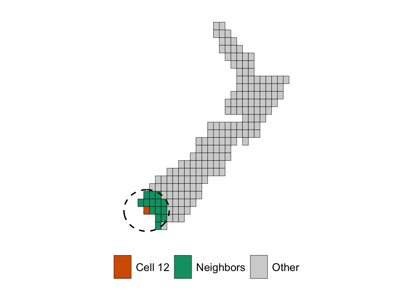
For example, for cell ID 12, the cells within 150km radius:

example_nn <- find_neighbors_radius(id = 12, 150*1000)
example_nn

# A tibble: 14 × 3
   cell_id cell_id_neighbors distance
     <dbl>             <int>    <dbl>
 1      12                19   38446.
 2      12                13   55597.
 3      12                 9   67695.
 4      12                20   67695.
 5      12                29   76893.
 6      12                28   94601.
 7      12                30   95169.
 8      12                14  111194.
 9      12                39  115338.
10      12                21  117767.
11      12                38  127563.
12      12                40  128510.
13      12                27  134789.
14      12                31  135586.

Code

create_circle <- function(long, lat, radius){ 
  tibble(degree = 1:360) |> 
    rowwise() |> 
    mutate(
      long = geosphere::destPoint(c(long, lat), degree, radius)[1],
      lat = geosphere::destPoint(c(long, lat), degree, radius)[2]
    ) |> 
    ungroup()
}

cell_of_interest <- centroids_cells |> filter(cell_id == 12)
circle_sf <- create_circle(
  long = cell_of_interest$longitude,
  lat = cell_of_interest$latitude,
  radius = 150*1000
) |> 
  st_as_sf(coords = c("long", "lat"), crs = sf::st_crs(centroids_cells)) |> 
  summarise(geometry = st_combine(geometry)) %>% 
  st_cast("POLYGON")

ggplot() +
  geom_sf(
    data = cells_sf |> 
      mutate(
        type = case_when(
          cell_id == 12 ~ "Cell 12",
          cell_id %in% example_nn$cell_id_neighbors ~ "Neighbors",
          TRUE ~ "Other"
        )
      ),
    mapping = aes(fill = type),
    colour = "black"
  ) + 
  geom_sf(data = maps_level_0$NGA, fill = NA) +
  geom_sf(
    data = circle_sf, 
    color = "black", fill = NA, linewidth = .8, linetype = "dashed"
  ) +
  scale_fill_manual(
    NULL, 
    values = c("Cell 12" = "#D55E00", "Neighbors" = "#009E73", "Other" = "lightgray")
  ) +
  theme_map_paper() +
  theme(legend.position = "bottom")

Figure 4.4: Cells within a 150km radius from cell 12

Now, let us get all the neighbors of the cells with many missing values for min temperatures, and for max temperatures.

neighbors_precip <- 
  map(cell_id_missing_precip, ~find_neighbors_radius(id = .x, radius = 150*1000)) |> 
  list_rbind()

neighbors_tmin <- 
  map(cell_id_missing_tmin, ~find_neighbors_radius(id = .x, radius = 150*1000)) |> 
  list_rbind()

neighbors_tmax <- 
  map(cell_id_missing_tmax, ~find_neighbors_radius(id = .x, radius = 150*1000)) |> 
  list_rbind()

We then define the impute_na_neighbor_cells() function that identifies the values of a metric of interest (argument name_col) from the neighbor (found in argument neighbors) cells of a given cell (whose ID is given to the argument id).

#' @param id cell ID
#' @param neighbors tibble with distances of the neighbors (obtained with 
#'  `find_neighbors_radius()`)
#' @param name_col name of the columns in `country_weather_daily` to use to 
#'  impute data (from neighbors)
impute_na_neighbor_cells <- function(id, neighbors, name_col) {
  country_weather_daily |> filter(cell_id == !!id) |> 
    left_join(neighbors, relationship = "many-to-many", by = "cell_id") |> 
    left_join(
      country_weather_daily |>
        select(
          cell_id_neighbors = cell_id, 
          date,
          new_val_neighbors = !!sym(name_col)
        ) |> 
        sf::st_drop_geometry(),
      by = c("date", "cell_id_neighbors")
    ) |> 
    select(date, cell_id, cell_id_neighbors, new_val_neighbors, distance) |> 
    filter(!is.na(new_val_neighbors)) |> 
    group_by(cell_id, date) |> 
    mutate(weight_distance = distance / sum(distance)) |> 
    mutate(new_val_neighbors = new_val_neighbors * weight_distance) |> 
    summarise(
      new_val_neighbors = sum(new_val_neighbors),
      .groups = "drop"
    )
}

We apply this function to the cells for which many missing values were found, to impute values for min temperatures, and then for max temperatures.

neighbors_precip_new_val <- 
  map(
    cell_id_missing_precip, 
    ~impute_na_neighbor_cells(
      .x, neighbors = neighbors_precip, name_col = "precip_new")
  ) |> 
  list_rbind()

neighbors_tmin_new_val <- 
  map(
    cell_id_missing_tmin, 
    ~impute_na_neighbor_cells(
      .x, neighbors = neighbors_tmin, name_col = "tmin_new")
  ) |> 
  list_rbind()

neighbors_tmax_new_val <- 
  map(
    cell_id_missing_tmax, 
    ~impute_na_neighbor_cells(
      .x, neighbors = neighbors_tmax, name_col = "tmax_new")
  ) |> 
  list_rbind()

We replace the missing values in the table with daily observations:

country_weather_daily <- 
  country_weather_daily |> 
  left_join(
    neighbors_precip_new_val |> rename(precip_neighbors = new_val_neighbors)
  ) |> 
  left_join(
    neighbors_tmin_new_val |> rename(tmin_neighbors = new_val_neighbors)
  ) |> 
  left_join(
    neighbors_tmax_new_val |> rename(tmax_neighbors = new_val_neighbors)
  ) |> 
  mutate(
    # If temporal interpolation was not enough, replace with spatially
    # interpolated values
    precip_new = ifelse(is.na(precip_new), precip_neighbors, precip_new),
    tmin_new = ifelse(is.na(tmin_new), tmin_neighbors, tmin_new),
    tmax_new = ifelse(is.na(tmax_new), tmax_neighbors, tmax_new)
  )

4.5 Second Temporal Interpolation

There are still missing values:

precip: 2015-05-19 to 2015-05-26,
tmin and tmax: 1983-04-25 to 1983-04-30 and 2015-05-21 to 2015-05-26.

country_weather_daily |> filter(is.na(precip_new)) |> count(date)
country_weather_daily |> filter(is.na(tmin_new)) |> count(date)
country_weather_daily |> filter(is.na(tmax_new)) |> count(date)

For those observations, we use, again, a temporal interpolation. This time, we increase the windows’ width to 10 days.

country_weather_daily <- 
  country_weather_daily |> 
  arrange(date) |> 
  nest(.by = cell_id) |> 
  mutate(
    precip_new_2 = map(data, ~{
      if (sum(is.na(.x$precip_new)) >= nrow(.x)-1) {
        new_val <- NA
      } else {
        new_val <- imputeTS::na_interpolation(.x$precip_new, maxgap = 10, option = "spline")
      }
      new_val}
    ),
    tmin_new_2 = map(data, ~{
      if (sum(is.na(.x$tmin_new)) >= nrow(.x)-1) {
        new_val <- NA
      } else {
        new_val <- imputeTS::na_interpolation(.x$tmin_new, maxgap = 10, option = "spline")
      }
      new_val}
    ),
    tmax_new_2 = map(data, ~{
      if (sum(is.na(.x$tmax_new)) >= nrow(.x)-1) {
        new_val <- NA
      } else {
        new_val <- imputeTS::na_interpolation(.x$tmax_new, maxgap = 10, option = "spline")
      }
      new_val}
    )
  ) |> 
  unnest(cols = c(data, precip_new_2, tmin_new_2, tmax_new_2)) |> 
  mutate(
    precip_new_2 = ifelse(precip_new_2 < 0, 0, precip_new_2),
    precip_new = ifelse(is.na(precip_new), precip_new_2, precip_new),
    tmin_new = ifelse(is.na(tmin_new), tmin_new_2, tmin_new),
    tmax_new = ifelse(is.na(tmax_new), tmax_new_2, tmax_new)
  )

Lastly, we remove the raw values with missing data with the columns in which missing data were replaced.

country_weather_daily <- 
  country_weather_daily |> 
  dplyr::select(
    -precip, -tmin, -tmax, 
    -precip_neighbors, -tmin_neighbors, -tmax_neighbors,
    -precip_new_2, -tmin_new_2, -tmax_new_2
  ) |> 
  rename(precip = precip_new, tmin = tmin_new, tmax = tmax_new)

Let us save the results for later use.

save(
  country_weather_daily,
  file = "../data/Weather/CPC/NZL_daily_weather_corrected.rda"
)

Each row gives three metrics for a grid cell identified with its ID (cell_id) whose centroid’s coordinates are given in longitude and latitude, at a given day (date). The country the data refer to (Nigeria) is stated in column country_code. The metrics are total rainfall (precip), minimum temperature (tmin) and maximum temperature (tmax).

The content of this dataset is summarized in Table 4.1.

Table 4.1: Data dictionary for NGA_daily_weather_corrected.rda

Variable name	Type	Description
`longitude`	numeric	Longitude of the centroid of the cell
`latitude`	numeric	Latitude of the centroid of the cell
`country_code`	numeric	Country code (ISO 3166-1 alpha-3 code)
`date`	date	Date of the observation (YYYY-MM-DD)
`cell_id`	integer	Unique identifier of the cells of the grid
`precip`	numeric	Total rainfall, in mm
`tmin`	numeric	Minimum temperature, in °C
`tmax`	numeric	Maximum temperature, in °C