6  Merge With Macroeconomic Data

Objectives of this page

In this page, three types of data are merged into a single dataset that will later be used to analyze the response of the economy to a weather shock, using both a VAR model (Chapter 8) and a DSGE model (Chapter 10).

The first part introduces functions for seasonal adjustment, considering three alternative methods:

1. Using the X-13ARIMA-SEATS software,
2. Estimating a trend with a Hodrick–Prescott filter,
3. Estimating a linear trend with an ordinary least squares model.

The subsequent parts describe how we:

• Import and pre-process the rest-of-world data (Section 6.2),
• Load the national macroeconomic variables (Section 6.3),
• Import the weather data (Section 6.4).

These datasets are then merged into a single panel (Section 6.5), after which detrending functions are applied and all variables are transformed into real, per-capita terms (Section 6.6).

library(tidyverse)

── Attaching core tidyverse packages ──────────────────────── tidyverse 2.0.0 ──
✔ dplyr     1.1.4     ✔ readr     2.1.5
✔ forcats   1.0.0     ✔ stringr   1.5.2
✔ ggplot2   4.0.0     ✔ tibble    3.3.0
✔ lubridate 1.9.4     ✔ tidyr     1.3.1
✔ purrr     1.1.0     
── Conflicts ────────────────────────────────────────── tidyverse_conflicts() ──
✖ dplyr::filter() masks stats::filter()
✖ dplyr::lag()    masks stats::lag()
ℹ Use the conflicted package (<http://conflicted.r-lib.org/>) to force all conflicts to become errors

library(readxl)

Let us load the graphs theme functions (See Chapter 1):

source("../scripts/functions/utils.R")

6.1 Functions for Seasonal Adjustment

We define a function, remove_seasonality() as a wrapper to the seas() function from {seasonal}. This function uses X-13ARIMA-SEATS, the seasonal adjustment software developed by the United States Census Bureau, to remove seasonality of a column in a tibble.

#' Remove seasonality (or return trend) using X-13ARIMA-SEATS
#'
#' @param data A data frame.
#' @param var The column in `data` to adjust (unquoted or string).
#' @param start Start time for the `ts()` (e.g., c(1999, 1)).
#' @param freq Frequency of the series (default 4 = quarterly).
#'
#' @return A tibble with columns: year, quarter, YEARS, and the adjusted series.
remove_seasonality <- function(data, 
                               variable, 
                               start, 
                               freq = 4) {
  
  if (!freq %in% c(4, 12)) {
    stop("`freq` must be either 4 (quarterly) or 12 (monthly).", call. = FALSE)
  }
  v_sym <- rlang::ensym(variable)
  v_name <- rlang::as_name(v_sym)
  
  # Turn in a ts object
  data_ts <- data |> pull(v_sym) |> 
    stats::ts(start = start, frequency = freq)
  
  # X-13ARIMA-SEATS
  fit <- seasonal::seas(data_ts)
  # Extract trend (seasonaly adjuster series)
  trend <- seasonal::final(fit)
  time_data <- stats::time(data_ts)
  
  if (freq == 4) {
    time_data <- zoo::as.yearqtr(time_data)
    res <- tibble::tibble(
      year = as.numeric(format(time_data, "%Y")),
      quarter = as.numeric(format(time_data, "%q")),
      !!v_name := trend
    ) |>
      dplyr::mutate(
        YEARS = year + c(0, 0.25, 0.5, 0.75)[quarter]
      )
  } else if (freq == 12) {
    time_data_q <- zoo::as.yearqtr(time_data)
    time_data <- zoo::as.yearmon(time_data)
    res <- tibble::tibble(
      year = as.numeric(format(time_data, "%Y")),
      month = as.numeric(format(time_data, "%m")),
      quarter = as.numeric(format(time_data_q, "%q")),
      !!v_name := trend
    ) |>
      dplyr::mutate(
        YEARS = as.numeric(time_data)
      )
  }
  
  res
}

We also define another functions to remove trend: myfilter(). It calls one of the two other functions we define, hp_filter() or lin_trend() to remove seasonality in a series. With hp_filter() we use a Hodrick-Prescott filter from {mFilter} (using \(\lambda=1600\), for quarterly data). With lin_trend(), we estimate a linear trend and return it.

#' Detrends a time serie
#' 
#' @param x Serie to be detrended (numeric).
#' @param type Type of the method applied: Hodrick-Prescott (hp) of OLS (ols).
myfilter <- function(x, type = c("hp", "ols")) {

  if (type == "hp") {
    res <- hp_filter(x)
    res <- log(x / res) * 100
  } else if (type == "ols") {
    x_log <- log(x)*100
    trend_x <- lin_trend(x_log)
    res <- x_log - trend_x
  } else {
    stop("Not the right filter")
  }
  res
}

#' Applies the HP filter on a quarterly time serie
#' 
#' @param x Series for which to retrieve the trend.
#' @returns The trend part of the series.
#' 
#' @importFrom mFilter hpfilter
#' 
hp_filter <- function(x) {
  serie <- x
  if (any(is.na(x))) {
    serie <- x[!is.na(x)]
  }
  
  res <- mFilter::hpfilter(serie, freq = 1600, type = "lambda")$trend |> as.vector()
  if (any(is.na(x))) {
    x[!is.na(x)] <- res
    res <- x
  }
  res
}

#' Returns the linear trend of `x`
#' 
lin_trend <- function(x, trend_val = df$YEARS) {
  
  serie <- x
  if (any(is.na(x))) {
    serie <- x[!is.na(x)]
    trend_val <- trend_val[!is.na(x)]
  }
  
  df_tmp <- data.frame(x = serie) |> 
    mutate(cste = 1, trend = trend_val)
  
  reg <- lm(x ~ 1 + trend, data = df_tmp)
  resul <- coef(reg)[["trend"]]*df_tmp$trend + coef(reg)[["(Intercept)"]]
  
  
  if (any(is.na(x))) {
    x[!is.na(x)] <- resul
    resul <- x
  }
  
  resul
}

6.2 Trading Partners

In Chapter 8, we will estimate a VAR model with three blocks:

• Weather block: captures climate variability indicators.
• Trading partners’ block: represents external economic shocks.
• Domestic economy block: corresponds to New Zealand.

New Zealand is a small open economy, meaning that its business cycles are influenced by shocks affecting its main trading partners.

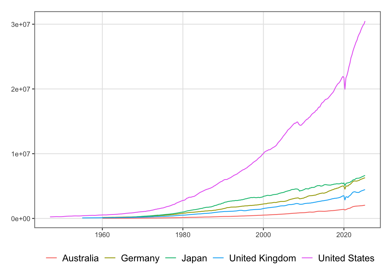
To account for these external effects, we construct a synthetic rest-of-world GDP based on the top five partners: Australia, Germany, Japan, the United Kingdom, and the United States.

The following macroeconomic series are imported for each country:

Table 6.1: Source of the different macroeconomic series

Variable	Source	Frequency	Purpose
Gross domestic product	OECD QNA	Quarterly	Economic conditions
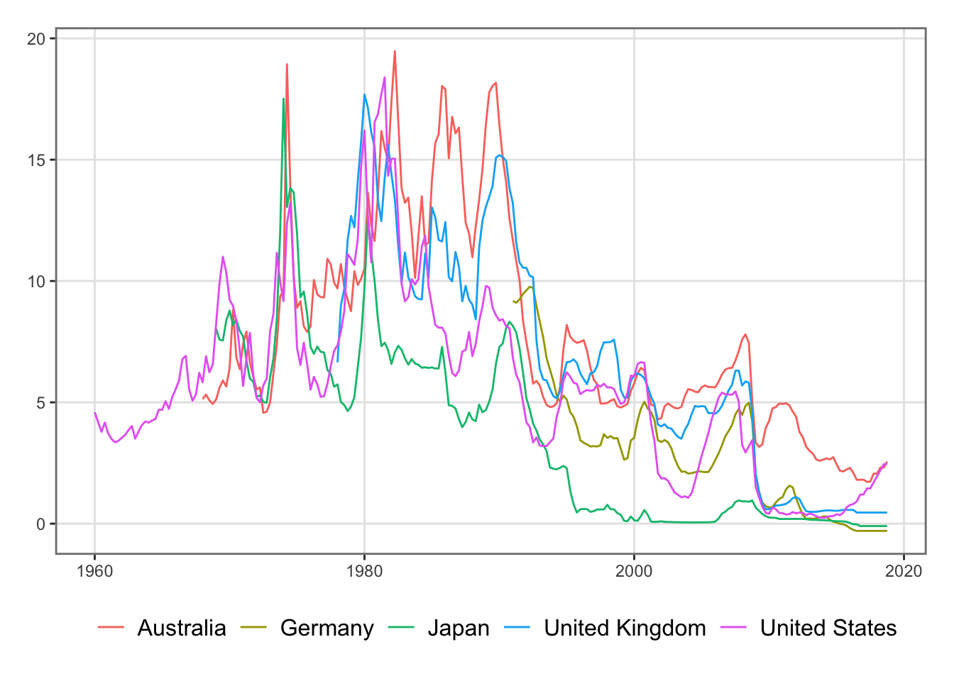
Short-term interest rate	OECD EO100	Quarterly	Global monetary stance
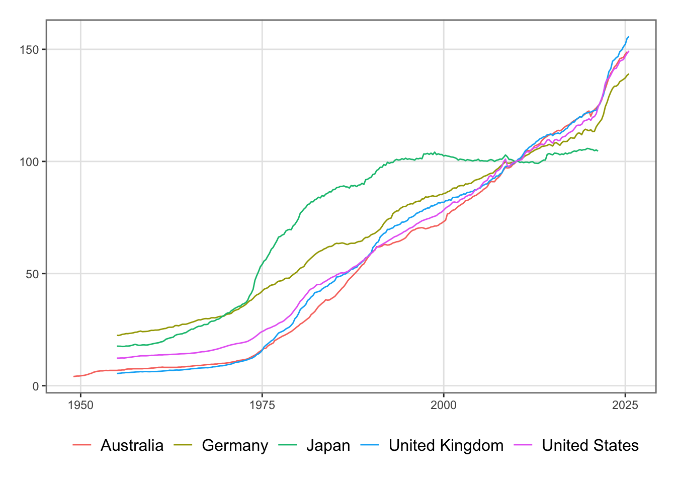
Consumer Price Index (CPI)	OECD QNA	Quarterly	Inflation proxy
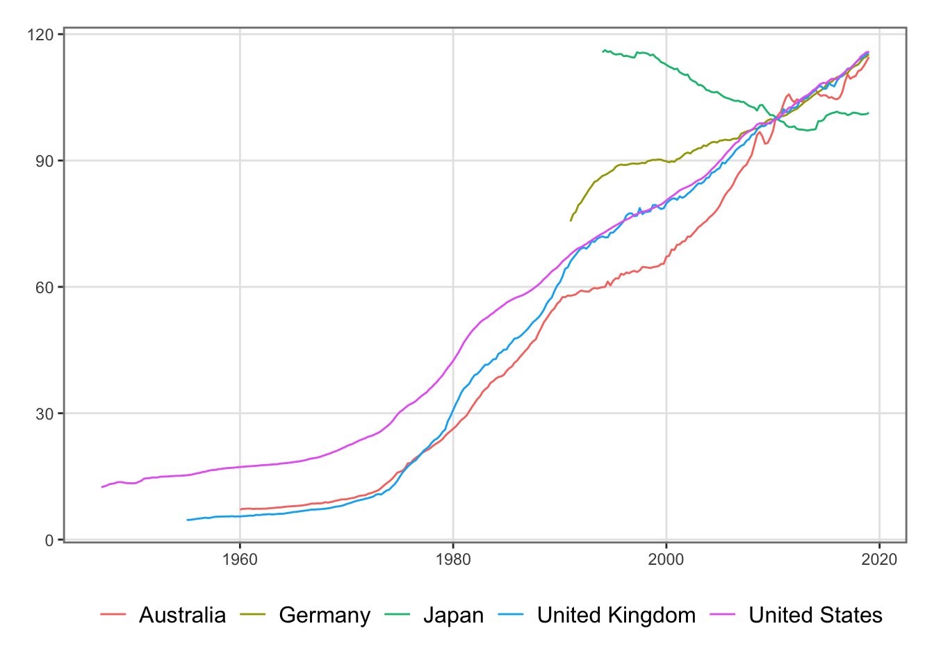
GDP Deflator	OECD QNA archive	Quarterly	Price base consistency
Population (15–64)	OECD historical population data	Annual → Quarterly	Scaling variable

The series are in Excel files in ../data/Economic/Rest-world. In the codes that follow, we harmonize them and, when necessary, rebase them to 2010 = 100. Annual population data are converted to quarterly frequency using the Denton–Cholette disaggregation method.

We set a reference year for the index:

ref_year <- 2010

6.2.1 Gross Domestic Product

• Source: OECD
• Quarterly GDP and components - expenditure approach, US Dollars
• Frequency of observation: Quarterly
• Price base: Current prices
• Combined transaction: Gross domestic product, Total economy

df_gdp <- read_excel(
  "../data/Economic/Rest-world/GDP.xlsx", skip = 5,
  n_max = 6
) |> 
  select(-`Time period...2`,-`Time period...3`) |> 
  rename(country = `Time period...1`) |> 
  filter(country != "Reference area") |> 
  pivot_longer(cols = -country, values_to = "gdp") |> 
  mutate(
    year = str_sub(name, 1, 4) |> as.numeric(),
    quarter = str_sub(name, -1) |> as.numeric(),
    YEARS = year + (quarter-1)/4
  ) |> 
  select(-name)

p <- ggplot(
  data = df_gdp, 
  mapping = aes(x = YEARS, y = gdp, colour = country)
) +
  geom_line() +
  labs(x = NULL, y = NULL) +
  scale_colour_discrete(name = "") +
  theme_paper()
p

Warning: Removed 188 rows containing missing values or values outside the scale range
(`geom_line()`).

Figure 6.1: GDP (PPP, millions $, constant 2010 prices)

6.2.2 Interest Rate

• Source: OECD
• Economic Outlook No 100 - November 2016
• Variable: Short-term interest rate
• Frequency: Quarterly
• https://stats.oecd.org/Index.aspx?DataSetCode=EO100_INTERNET

df_r <- read_excel(
  "../data/Economic/Rest-world/interest-rate.xlsx",
  skip = 4, n_max = 6
) |> 
  select(-`Time...2`) |> 
  rename(country = `Time...1`) |> 
  filter(country != "Country") |> 
  pivot_longer(cols = -country, values_to = "r") |> 
  mutate(
    year = str_sub(name, 1, 4) |> as.numeric(),
    quarter = str_sub(name, -1) |> as.numeric(),
    YEARS = year + (quarter-1)/4
  ) |> 
  select(-name)

New names:
• `Time` -> `Time...1`
• `Time` -> `Time...2`

p <- ggplot(
  data = df_r, 
  mapping = aes(x = YEARS, y = r, colour = country)
) +
  geom_line() +
  labs(x = NULL, y = NULL) +
  scale_colour_discrete(name = "") +
  theme_paper()
p

Warning: Removed 264 rows containing missing values or values outside the scale range
(`geom_line()`).

Figure 6.2: Short-Term Interest Rate

Remove missing observation.

df_r <- df_r |>  filter(!is.na(r))

6.2.3 Consumer Price Index

• Source: OECD
• Consumer price indices (CPIs, HICPs), COICOP 1999
• Frequency of observation: Quarterly
• Measure: Consumer price index, National
• Unit of measure: Index, 2015

df_cpi <- read_excel(
  "../data/Economic/Rest-world/CPI.xlsx",
  skip = 5, n_max = 6
) |> 
  select(-`Time period...2`) |> 
  rename(country = `Time period...1`) |> 
  filter(country != "Reference area") |> 
  pivot_longer(cols = -country, values_to = "cpi") |> 
  mutate(
    year = str_sub(name, 1, 4) |> as.numeric(),
    quarter = str_sub(name, -1) |> as.numeric(),
    YEARS = year + (quarter-1)/4
  ) |> 
  select(-name)

Change base year:

ref_cpi <- df_cpi |>  
  filter(YEARS == !!ref_year) |> 
  select(country, cpi_ref = cpi)

df_cpi <- df_cpi |> 
  left_join(ref_cpi, by = c("country")) |> 
  mutate(
    cpi = cpi / cpi_ref * 100
  ) |> 
  select(-cpi_ref)

p <- ggplot(
  data = df_cpi, 
  mapping = aes(x = YEARS, y = cpi, colour = country)
) +
  geom_line() +
  labs(x = NULL, y = NULL) +
  scale_colour_discrete(name = "") +
  theme_paper()
p

Warning: Removed 114 rows containing missing values or values outside the scale range
(`geom_line()`).

Figure 6.3: CPI

Remove missing obs.

df_cpi <- df_cpi |> filter(!is.na(cpi))

6.2.4 GDP Deflator

• Source: OECD
• QNA – Archive before 2019 benchmark revisions
• Subject: Gross domestic product - expenditure approach
• Measure: Deflator, OECD reference year, seasonally adjusted
• Frequency: Quarterly

df_gdp_defl <- read_excel(
  "../data/Economic/Rest-world/GDP_deflator.xlsx",
  skip = 4, n_max = 7
) |> 
  select(-`Period...2`) |> 
  rename(country = `Period...1`) |> 
  filter(country != "Country") |> 
  pivot_longer(cols = -country, values_to = "gdp_defl") |> 
  mutate(
    year = str_sub(name, 1, 4) |> as.numeric(),
    quarter = str_sub(name, -1) |> as.numeric(),
    YEARS = year + (quarter-1)/4
  ) |> 
  select(-name)

p <- ggplot(
  data = df_gdp_defl, 
  mapping = aes(x = YEARS, y = gdp_defl, colour = country)
) +
  geom_line() +
  labs(x = NULL, y = NULL) +
  scale_colour_discrete(name = "") +
  theme_paper()
p

Warning: Removed 448 rows containing missing values or values outside the scale range
(`geom_line()`).

Figure 6.4: GDP Deflator

Remove missing values:

df_gdp_defl <- df_gdp_defl |>  filter(!is.na(gdp_defl))

6.2.5 Population

• Source: OECD
• Historical population data
• Measure: Population
• Age: From 15 to 64 years
• Time horizon: Historical
• Combined unit of measure: Persons

pop <- read_excel(
  "../data/Economic/Rest-world/pop.xlsx", skip = 5,
  n_max = 7
) |> 
  select(-`Time period...2`) |> 
  rename(country = `Time period...1`) |> 
  filter(country != "Reference area") |> 
  pivot_longer(cols = -country, values_to = "pop") |> 
  mutate(
    year = str_sub(name, 1, 4) |> as.numeric()
  ) |> 
  select(-name)

The population data is given at an annual rate. We use the Denton-Cholette method to estimate quarterly values, thanks to the td() function from {tempdisagg}. We define a function, pop_quarterly() as a wrapper function to do so, for a specific country.

library(tempdisagg)

#' Estimate quarterly population from annual values
#' 
#' @param country Name of the country in the dataset `pop`.
#' 
pop_quarterly <- function(country) {
  x <- pop |> 
    filter(country %in% !!country)
  x_ts <- ts(x$pop, start = as.numeric(x$year[1]))
  # Forecast 3 years ahead
  x_f <- forecast::forecast(forecast::auto.arima(x_ts), h = 3)
  # Disaggregate
  x_ts <- ts(c(x_ts, x_f$mean), start = start(x_ts))
  res <- predict(td(x_ts ~ 1, method = "denton-cholette", conversion = "average"))
  res <- tibble(
    YEARS = as.vector(time(res)), 
    country = country, 
    pop = as.vector(res)
  )
  
  # Change base year
  ref_pop <- res |> filter(YEARS == ref_year) |> pull("pop")
  
  res |> mutate(pop = pop / ref_pop * 100)
}

We apply the pop_quarterly() on each of the trading partner’s population data.

df_pop <- 
  map(unique(pop$country), ~pop_quarterly(.x)) |> 
  list_rbind()

Registered S3 method overwritten by 'quantmod':
  method            from
  as.zoo.data.frame zoo 

p <- ggplot(
  data = df_pop, 
  mapping = aes(x = YEARS, y = pop, colour = country)
) +
  geom_line() +
  labs(x = NULL, y = NULL) +
  scale_colour_discrete(name = "") +
  theme_paper()
p

Figure 6.5: Population

Remove missing values:

df_pop <- df_pop |>  filter(!is.na(pop))

6.2.6 GDP, Inflation rate, and CPI

The quarterly share of each country’s GDP can be easily computed:

shares <- 
  df_gdp |> 
  group_by(year, quarter, YEARS) |> 
  mutate(total_gdp = sum(gdp)) |> 
  ungroup() |> 
  filter(YEARS >= 1987, YEARS < 2017) |> 
  mutate(share = gdp / total_gdp) |> 
  select(YEARS, country, share)

Let us merge all the previous series in a single dataset.

df_row_raw <- 
  df_gdp |> 
  left_join(df_r, by = c("country", "year", "quarter", "YEARS")) |> 
  left_join(df_cpi, by = c("country", "year", "quarter", "YEARS")) |> 
  left_join(df_gdp_defl, by = c("country", "year", "quarter", "YEARS")) |> 
  left_join(df_pop, by = c("country", "YEARS")) |> 
  left_join(shares, by = c("country", "YEARS")) |> 
  rename(years = YEARS) |> 
  filter(years >= 1987, years < 2017) |> 
  mutate(prices = gdp_defl)

We express the values in per-capita real terms.

df_w <- 
  df_row_raw |> 
  mutate(r_y = gdp / pop / prices) |> 
  mutate(
    r_y = r_y * share,
    cpi = cpi * share,
    gdp_defl = gdp_defl * share,
    r = r * share
  ) |> 
  group_by(years) |> 
  summarise(
    wgdp = sum(r_y),
    wcpi = sum(cpi),
    wgdp_def = sum(gdp_defl),
    wr = sum(r),
    .groups = "drop"
  ) |> 
  rename(YEARS = years)

df_w

# A tibble: 120 × 5
   YEARS  wgdp  wcpi wgdp_def    wr
   <dbl> <dbl> <dbl>    <dbl> <dbl>
 1 1987     NA  60.4       NA    NA
 2 1987.    NA  61.1       NA    NA
 3 1988.    NA  61.5       NA    NA
 4 1988.    NA  61.9       NA    NA
 5 1988     NA  62.2       NA    NA
 6 1988.    NA  62.7       NA    NA
 7 1988.    NA  63.3       NA    NA
 8 1989.    NA  63.9       NA    NA
 9 1989     NA  64.4       NA    NA
10 1989.    NA  65.5       NA    NA
# ℹ 110 more rows

6.3 Macroeconomic Variables

The macroeconomic variables are in an Excel file:

excel_file <- "../data/Economic/data_nz.xls"

6.3.1 GDP (All industries & Agriculture)

• GDP (All industries & Agriculture)—-
• Seasonnaly adjusted
• Source: OECD
• Frequency: quarterly

gdp <- readxl::read_excel(path = excel_file, sheet = "Y", skip = 2)

gdp <- gdp |> 
  dplyr::select(
    date, 
    `NZNTAGCL Index`, # Agriculture Chain Volume
    `NZNTPRAS Index`, # GDP Chain Volume
    `NZNTNOM Index`   # NZ Expenditure Based GDP (Nominal, SA, NZD)
  ) |> 
  mutate(
    agri_share = `NZNTAGCL Index` / `NZNTPRAS Index`,
    gdp_a = agri_share * `NZNTNOM Index`
  ) |> 
  rename(gdp_tot = `NZNTNOM Index`) |> 
  mutate(
    gdp = gdp_tot - gdp_a,
    year = as.numeric(str_sub(date, 1, 4)),
    quarter = as.numeric(str_sub(date, 6, 7)),
    quarter = ceiling(quarter / 3),
    YEARS = year + quarter / 4 - 0.25
  ) |> 
  select(YEARS, gdp, gdp_a, gdp_tot)

6.3.2 Consumption

• Source: Statistics New Zealand
• Frequency: quarterly

consum <- readxl::read_excel(
  path = excel_file, sheet = "C", skip = 3
) |> 
  rename(
    YEARS = `...1`,
    c = `Households...2`,
    c_a = `Households...3`
  )

consum <- 
  consum |> 
  select(YEARS, c, c_a) |> 
  filter(YEARS %>% str_detect("^[[:alnum:]]{4}Q[[:alnum:]]$")) |> 
  mutate(
    year = as.numeric(str_sub(YEARS, 1, 4)),
    quarter = c(0, 0.25, 0.5, 0.75)[as.numeric(str_sub(YEARS, -1))],
    YEARS = year + quarter,
    c = c |> as.character() |> as.numeric(),
    c_a = c_a |> as.character() |> as.numeric()
  ) |> 
  select(-year, -quarter)

6.3.3 Investment

• Source: Statistics New Zealand
• Frequency: quarterly

invest <- readxl::read_excel(path = excel_file, sheet = "inv") |> 
  rename(
    YEARS = Series,
    I = `GDP(E)`,
    I_private = Nominal
  )


invest <- 
  invest |> 
  select(YEARS, I,I_private) |> 
  filter(YEARS %>% str_detect("^[[:alnum:]]{4}Q[[:alnum:]]$")) |> 
  mutate(
    year = as.numeric(str_sub(YEARS, 1, 4)),
    quarter = c(0, 0.25, 0.5, 0.75)[as.numeric(str_sub(YEARS, -1))],
    YEARS = year + quarter,
    I = I |>  as.character() |>  as.numeric(),
    I_private = I_private |> as.character() |>  as.numeric()
  ) |> 
  select(-year, -quarter)

6.3.4 Consumer price index

• Source: Statistics New Zealand
• Frequency: quarterly

cpi <- readxl::read_excel(path = excel_file, sheet = "CPI", skip = 1, na = ",,"
) |> 
  rename(
    YEARS = `...1` ,
    P = `All groups`
  )

cpi <- 
  cpi |> 
  select(YEARS, P) |> 
  filter(YEARS |> str_detect("^[[:digit:]]{4}Q[[:digit:]]$")) |> 
  mutate(
    year = as.numeric(str_sub(YEARS, 1, 4)),
    quarter = c(0, 0.25, 0.5, 0.75)[as.numeric(str_sub(YEARS, -1))],
    YEARS = year + quarter
  ) |> 
  select(-year, -quarter) |> 
  mutate(P = P |>  as.character() |> as.numeric())

Warning: There was 1 warning in `mutate()`.
ℹ In argument: `P = as.numeric(as.character(P))`.
Caused by warning:
! NAs introduced by coercion

Change base year:

ref_cpi <- cpi |>  filter(YEARS == ref_year) |>  pull("P")

cpi <- 
  cpi |> 
  mutate(P = P / ref_cpi * 100)

6.3.5 GDP Deflator

• Source: Statistics New Zealand
• Frequency: quarterly

gdp_defl <- readxl::read_excel(path = excel_file, sheet = "CPI", skip = 1, na = ",,"
) |> 
  select(years, gdp_defl)


gdp_defl <- 
  gdp_defl |> 
  filter(years %>% str_detect("^[[:digit:]]{4}Q[[:digit:]]$")) |> 
  mutate(
    year = as.numeric(str_sub(years, 1, 4)),
    quarter = c(0, 0.25, 0.5, 0.75)[as.numeric(str_sub(years, -1))],
    years = year + quarter
  ) |> 
  select(-year, -quarter) |> 
  rename(YEARS = years, PP = gdp_defl) |> 
  mutate(PP = PP |> as.character() |> as.numeric())

# Change base year
ref_pp <- gdp_defl |> filter(YEARS == ref_year) |> pull("PP")

gdp_defl <- 
  gdp_defl |> 
  mutate(PP = PP / ref_pp * 100)

6.3.6 Exports

• Source: OECD
• Frequency: quarterly

trade <- readxl::read_excel(
  path = excel_file, sheet = "imports_exports", skip = 3, na = ",,"
)

trade <- 
  trade |> 
  filter(YEARS %>% str_detect("^[[:digit:]]{4}Q[[:digit:]]$")) |> 
  mutate(
    year = as.numeric(str_sub(YEARS, 1, 4)),
    quarter = c(0, 0.25, 0.5, 0.75)[as.numeric(str_sub(YEARS, -1))],
    YEARS = year + quarter
  ) |> 
  select(-year, -quarter) |> 
  mutate(
    exports_a = as.numeric(as.character(exports_a)),
    imports = as.numeric(as.character(imports_sa_vfd)),
    exports = as.numeric(as.character(exports_sa))
  )

6.3.7 Paid hours

• Source: Statistics New Zealand
• Frequency: quarterly

paid_hours <- readxl::read_excel(
  path = excel_file, sheet = "Hours(FTE)", skip = 1, na = ",,"
) |> 
  rename(
    YEARS = `...1`,
    weekly = `Total All Industries`
  )

paid_hours <- 
  paid_hours |> 
  select(YEARS, weekly) |> 
  filter(YEARS |> str_detect("^[[:digit:]]{4}Q[[:digit:]]$")) |> 
  mutate(
    year = as.numeric(str_sub(YEARS, 1, 4)),
    quarter = c(0, 0.25, 0.5, 0.75)[as.numeric(str_sub(YEARS, -1))],
    YEARS = year + quarter
  ) |> 
  select(-year, -quarter) |> 
  rename(H = weekly) |> 
  mutate(H = as.numeric(as.character(H)))

Index:

ref_hours <- paid_hours |> filter(YEARS == ref_year) |> pull("H")

paid_hours <- 
  paid_hours |> 
  mutate(H = H / ref_hours * 100)

6.3.8 Employment

• Source: Statistics New Zealand
• Frequency: quarterly

employment <- readxl::read_excel(
  path = excel_file, sheet = "employment", skip = 2, na = ",,"
) |> 
  rename(employment = `Employment Rate`)


employment <- 
  employment |> 
  select(YEARS, employment) |> 
  filter(YEARS %>% str_detect("^[[:digit:]]{4}Q[[:digit:]]$")) |> 
  mutate(
    year = as.numeric(str_sub(YEARS, 1, 4)),
    quarter = c(0, 0.25, 0.5, 0.75)[as.numeric(str_sub(YEARS, -1))],
    YEARS = year + quarter
  ) |> 
  select(-year, -quarter) |> 
  rename(E = employment) |> 
  mutate(E = as.numeric(as.character(E)))

6.3.9 Wages

• Source: Statistics New Zealand
• Frequency: quarterly

wages <- readxl::read_excel(
  path = excel_file, sheet = "Wages", skip = 3, na = ",,"
) |> 
  rename(
    YEARS = `...1`,
    Wage = `Total - Seasonally Adjusted`
  )

wages <- 
  wages |> 
  select(YEARS, Wage) |> 
  filter(YEARS |> str_detect("^[[:digit:]]{4}Q[[:digit:]]$")) |> 
  mutate(
    year = as.numeric(str_sub(YEARS, 1, 4)),
    quarter = c(0, 0.25, 0.5, 0.75)[as.numeric(str_sub(YEARS, -1))],
    YEARS = year + quarter
  ) |> 
  select(-year, -quarter) |> 
  rename(W = Wage) |> 
  mutate(W = as.numeric(as.character(W)))

Change base year:

ref_wages <- wages |> filter(YEARS == ref_year) |> pull("W")

wages <- 
  wages |> 
  mutate(W = W / ref_wages * 100)

6.3.10 Population

• Source: Statistics New Zealand
• Frequency: quarterly

pop <- readxl::read_excel(path = excel_file, sheet = "POP", skip = 1)
colnames(pop)[c(1,2)] <- c("YEARS", "pop")

pop <- 
  pop |> 
  select(YEARS, pop) |> 
  mutate(POP = pop |> str_replace_all(",", "")) |> 
  select(-pop) |> 
  filter(YEARS |> str_detect("^[[:digit:]]{4}Q[[:digit:]]$")) |> 
  mutate(
    year = as.numeric(str_sub(YEARS, 1, 4)),
    quarter = c(0, 0.25, 0.5, 0.75)[as.numeric(str_sub(YEARS, -1))],
    YEARS = year + quarter,
    POP = POP |> as.character() |> as.numeric()
  ) |> 
  select(-year, -quarter)

As an index:

pop_ref <- pop |>  filter(YEARS == ref_year) |> pull("POP")

pop <- 
  pop |> 
  mutate(POP = POP / pop_ref)

6.3.11 Production prices

• Production prices (All industrie & agriculture)—-
• Source: Statistics New Zealand
• Frequency: quarterly

prices <- readxl::read_excel(
  path = excel_file, sheet = "productionPrice", skip = 1, na = ",,"
) |> 
  rename(
    YEARS = `...1`,
    P = `All Industries`,
    P_A = `Agriculture, Forestry and Fishing`
  )

prices <-
  prices |> 
  select(YEARS, P_A) |> 
  filter(YEARS |> str_detect("^[[:alnum:]]{4}Q[[:alnum:]]")) |> 
  mutate(
    year = as.numeric(str_sub(YEARS, 1, 4)),
    quarter = c(0, 0.25, 0.5, 0.75)[as.numeric(str_sub(YEARS, -1))],
    YEARS = year + quarter,
    P_A = P_A |> as.character() |> as.numeric()
  ) |> 
  select(-year, -quarter)

Price indices:

p_a_ref <- prices %>% filter(YEARS == ref_year) |> pull("P_A")

# Join CPI
prices <- 
  cpi |> 
  left_join(prices)

Joining with `by = join_by(YEARS)`

prices <- 
  prices |> 
  mutate(P_A = P_A / p_a_ref * 100)

# Join CPI
prices <- 
  cpi |> 
  left_join(prices)

Joining with `by = join_by(YEARS, P)`

6.3.12 Interest rate

• Source: OECD stat
• Frequency: quarterly

interest <- readxl::read_excel(
  path = excel_file, sheet = "R", na = ",,", skip = 10
) |> 
  select(YEARS = observation_date, R = IR3TBB01NZQ156N)

interest <- 
  interest |> 
  mutate(YEARS = YEARS |> ymd()) |> 
  mutate(
    year = year(YEARS),
    quarter = YEARS |> quarter(),
    YEARS = year + c(0, 0.25, 0.5, 0.75)[quarter]
  ) |> 
  select(-year, -quarter) |> 
  filter(!is.na(YEARS), str_length(YEARS) > 0)

6.3.13 Exchange Rate

• Source: FRED

ex_rate <- readxl::read_excel(
  path = excel_file, sheet = "ExchangeRate", skip = 0
)

ex_rate <- ex_rate[, which(colnames(ex_rate) %in% c("DATE", "RTWI"))]

ex_rate <- 
  ex_rate |> 
  mutate(
    quarter = str_extract(DATE, "M(.*?)$"),
    quarter = str_sub(quarter, 2),
    quarter = match(quarter, c(1,4, 7, 10)),
    year = str_sub(DATE, 1, 4) |> as.numeric(),
    YEARS = year + quarter/4 - 0.25
  ) |> 
  select(-quarter, -year, -DATE)

As an index:

ex_rate_ref <- ex_rate |> filter(YEARS == ref_year) |>  pull("RTWI")

ex_rate <-
  ex_rate |> 
  mutate(ex_rate = RTWI / ex_rate_ref * 100) |> 
  select(YEARS, ex_rate)

6.3.14 Real Effective Exchange Rate

• Source: FRED
• Real Broad Effective Exchange Rate for New Zealand (RBNZBIS)
• Source: Bank for International Settlements
• Not seasonally adjusted, monthly

reer <- readxl::read_excel(path = excel_file, sheet = "Reer", skip = 10)

Seasonal adjustment:

debut_reer <- reer$observation_date[1]

reer <- 
  remove_seasonality(
  data = reer, 
  variable = "RBNZBIS", 
  start = c(year(debut_reer), month(debut_reer)), 
  freq = 12
) |> 
  group_by(year, quarter) |> 
  summarise(reer = mean(RBNZBIS), .groups = "drop")

Model used in SEATS is different: (0 1 1)

Add years:

reer <-
  reer |> 
  mutate(YEARS = as.numeric(year) + as.numeric(quarter)/4 - 0.25) |> 
  select(-quarter, -year)

As an index:

reer_ref <- reer |> filter(YEARS == ref_year) |> pull("reer")

reer <-
  reer |> 
  mutate(reer = reer / reer_ref * 100) |> 
  select(YEARS, reer)

6.3.15 Share Price (OECD)

6.3.15.1 OECD

• Source : OECD

share_price <- readxl::read_excel(
  path = excel_file, sheet = "Share_Prices(OECD)", skip = 1
)

share_price <- 
  share_price |> 
  mutate(
    year = as.numeric(str_sub(YEARS, -4)),
    quarter = c(0, 0.25, 0.5, 0.75)[as.numeric(str_sub(YEARS, 2,2))],
    YEARS = year + quarter,
    share_price = share_prices_index |> as.character() |> as.numeric()
  ) |> 
  select(-year, -quarter)

As an index:

share_price_ref <- share_price |> filter(YEARS == ref_year) |> pull("share_price")

share_price <-
  share_price |> 
  mutate(share_price = share_price / share_price_ref * 100)

6.3.15.2 Bloomberg

• Source: BLOOMBERG

share_price <- readxl::read_excel(
  path = excel_file, sheet = "NZSE_Index", skip = 1
)

share_price <-
  share_price |> 
  rename(date = Date, share_price = PX_LAST) |> 
  mutate(
    year = year(date),
    month = month(date),
    quarter = match(month, c(3,6,9,12)),
    YEARS = year + quarter/4 - 0.25
  ) |> 
  select(YEARS, share_price)

As an index:

share_price_ref <- share_price |> 
  filter(YEARS == ref_year) |>
  pull("share_price")

share_price <-
  share_price |> 
  mutate(share_price = share_price / share_price_ref * 100)

6.3.16 Crude Oil Prices (Dubai)

• Source : FRED
• Global price of Dubai Crude,
• U.S. Dollars per Barrell, Quarterly, Not Seasonally Adjusted

crude_oil <- readxl::read_excel(
  path = excel_file, sheet = "Crude Oil", skip = 10
)

crude_oil <- 
  crude_oil |> 
  rename(date = observation_date, crude_oil = POILDUBUSDQ) |> 
  mutate(
    date = as.Date(date),
    year = year(date),
    month = month(date),
    quarter = match(month, c(1,4,7,10)),
    YEARS = year + quarter/4 - 0.25
  )

Adjust seasonality:

crude_oil_desais <- 
  remove_seasonality(
    data = crude_oil, 
    variable = "crude_oil", 
    start = c(crude_oil$year[1], crude_oil$quarter[1]),
    freq = 4
  )

Model used in SEATS is different: (0 1 1)

crude_oil <- 
  crude_oil |> 
  select(-crude_oil) |> 
  left_join(crude_oil_desais, by = "YEARS") |> 
  select(YEARS, crude_oil)

As an index:

crude_oil_ref <- crude_oil |> filter(YEARS == ref_year) |>  pull("crude_oil")

crude_oil <-
  crude_oil |> 
  mutate(crude_oil = crude_oil / crude_oil_ref * 100)

6.4 Weather data

The weather data obtained in Chapter 5 were saved in an Rdata file that can be loaded with the load() function.

load("../data/Weather/national_weather_quarterly.rda")

national_weather_quarterly <- 
  national_weather_quarterly |> 
  mutate(YEARS = year + quarter/4 - 0.25)

Warning

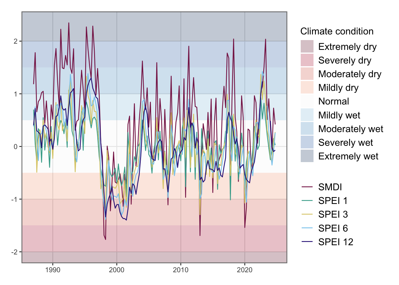
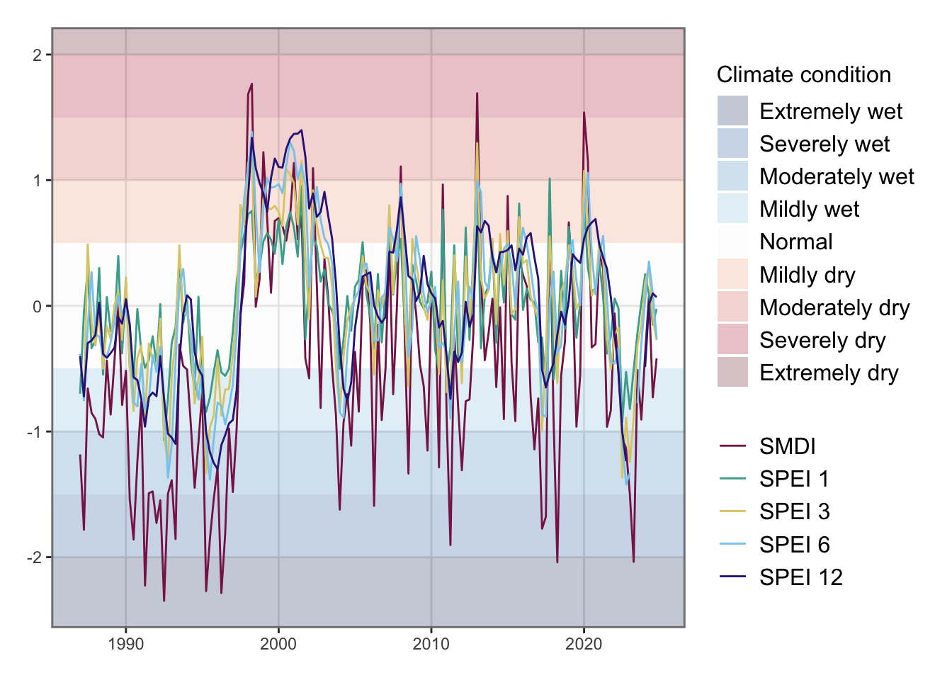
Negative values of the Soil Moisture Deficit index depict droughts (see Figure 6.6 ). In the impulse response functions, we will impulse positive standard deviation shocks. To depict a shock corresponding to a increase in dryness, we change the sign of the SMDI variable (see Figure 6.7).

spei_bands <- tibble(
  ymin = c(-Inf, -2.0, -1.5, -1.0, -0.5,  0.5,  1.0,  1.5,  2.0),
  ymax = c(-2.0, -1.5, -1.0, -0.5,  0.5,  1.0,  1.5,  2.0,  Inf),
  label = c(
    "Extremely dry", "Severely dry", "Moderately dry", "Mildly dry",
    "Normal",
    "Mildly wet", "Moderately wet", "Severely wet", "Extremely wet"
  ),
  fill = c(
    "#67001f", "#b2182b", "#d6604d", "#f4a582", # dry shades
    "#f7f7f7",
    "#92c5de", "#4393c3", "#2166ac", "#053061" # wet shades
  )
) |> 
  mutate(label = factor(label, levels = label))

ggplot(data = national_weather_quarterly |> 
         dplyr::select(YEARS, SMDI, SPEI_1, SPEI_3, SPEI_6, SPEI_12) |> 
         pivot_longer(cols = -YEARS) |> 
         mutate(
           name = factor(
             name, 
             levels = c("SMDI", "SPEI_1", "SPEI_3", "SPEI_6", "SPEI_12"),
             labels = c("SMDI", "SPEI 1", "SPEI 3", "SPEI 6", "SPEI 12")
             )
         ),
       mapping = aes(x = YEARS, y = value, colour = name)
) + 
  geom_rect(
    data = spei_bands,
    aes(
      xmin = -Inf, xmax = Inf,
      ymin = ymin, ymax = ymax,
      fill = label
    ),
    inherit.aes = FALSE,
    alpha = 0.25
  ) +
  geom_line() +
  labs(x = NULL, y = NULL) +
  scale_colour_manual(
    name = NULL,
    values = c(
      "SMDI" = "#882255", 
      "SPEI 1" = "#44AA99", 
      "SPEI 3" = "#DDCC77", 
      "SPEI 6" = "#88CCEE", 
      "SPEI 12" = "#332288"
    )
    ) +
  scale_fill_manual(
    name = "Climate condition",
    values = setNames(spei_bands$fill, spei_bands$label)
  ) +
  theme_paper() +
  theme(legend.position = "right", legend.direction = "vertical")

Figure 6.6: Drought indices. Negative values correspond to dry conditions, positive values correspond to wet conditions.

# Flip sign of drought indices
national_weather_quarterly <- 
  national_weather_quarterly |> 
  mutate(
    across(
      .cols = c(SMDI, SPEI_1, SPEI_3, SPEI_6, SPEI_12), 
      .fns = ~ - .x
    )
  )

The new series are shown in Figure 6.7.

spei_bands <- tibble(
  ymin = c(-Inf, -2.0, -1.5, -1.0, -0.5,  0.5,  1.0,  1.5,  2.0),
  ymax = c(-2.0, -1.5, -1.0, -0.5,  0.5,  1.0,  1.5,  2.0,  Inf),
  label = rev(c(
    "Extremely dry", "Severely dry", "Moderately dry", "Mildly dry",
    "Normal",
    "Mildly wet", "Moderately wet", "Severely wet", "Extremely wet"
  )),
  fill = rev(c(
    "#67001f", "#b2182b", "#d6604d", "#f4a582", # dry shades
    "#f7f7f7",
    "#92c5de", "#4393c3", "#2166ac", "#053061" # wet shades
  ))
) |> 
  mutate(label = factor(label, levels = label))

ggplot(data = national_weather_quarterly |> 
         dplyr::select(YEARS, SMDI, SPEI_1, SPEI_3, SPEI_6, SPEI_12) |> 
         pivot_longer(cols = -YEARS) |> 
         mutate(
           name = factor(
             name, 
             levels = c("SMDI", "SPEI_1", "SPEI_3", "SPEI_6", "SPEI_12"),
             labels = c("SMDI", "SPEI 1", "SPEI 3", "SPEI 6", "SPEI 12")
             )
         ),
       mapping = aes(x = YEARS, y = value, colour = name)
) + 
  geom_rect(
    data = spei_bands,
    aes(
      xmin = -Inf, xmax = Inf,
      ymin = ymin, ymax = ymax,
      fill = label
    ),
    inherit.aes = FALSE,
    alpha = 0.25
  ) +
  geom_line() +
  labs(x = NULL, y = NULL) +
  scale_colour_manual(
    name = NULL,
    values = c(
      "SMDI" = "#882255", 
      "SPEI 1" = "#44AA99", 
      "SPEI 3" = "#DDCC77", 
      "SPEI 6" = "#88CCEE", 
      "SPEI 12" = "#332288"
    )
    ) +
  scale_fill_manual(
    name = "Climate condition",
    values = setNames(spei_bands$fill, spei_bands$label)
  ) +
  theme_paper() +
  theme(legend.position = "right", legend.direction = "vertical")

Figure 6.7: Drought indices with sign flipped. Negative values correspond to wet conditions, positive values correspond to dry conditions.

6.5 Merge

Let us merge all the previous datasets in a single one.

donnees_brutes_nz <- 
  national_weather_quarterly |> 
  full_join(gdp) |>  
  full_join(consum) |>  
  full_join(trade) |>  
  full_join(invest) |>   
  full_join(prices) |>   
  full_join(gdp_defl) |>  
  full_join(interest) |>  
  full_join(ex_rate) |>  
  full_join(reer) |>  
  full_join(pop) |>  
  full_join(paid_hours) |>  
  full_join(employment) |>  
  full_join(wages) |>  
  full_join(df_w) |>  
  full_join(share_price) |>  
  full_join(crude_oil) |>  
  filter(YEARS >= 1994.25, YEARS < 2017)

Joining with `by = join_by(YEARS)`
Joining with `by = join_by(YEARS)`
Joining with `by = join_by(YEARS)`
Joining with `by = join_by(YEARS)`
Joining with `by = join_by(YEARS)`
Joining with `by = join_by(YEARS)`
Joining with `by = join_by(YEARS)`
Joining with `by = join_by(YEARS)`
Joining with `by = join_by(YEARS)`
Joining with `by = join_by(YEARS)`
Joining with `by = join_by(YEARS)`
Joining with `by = join_by(YEARS)`
Joining with `by = join_by(YEARS)`
Joining with `by = join_by(YEARS)`
Joining with `by = join_by(YEARS)`
Joining with `by = join_by(YEARS)`

df <- 
  donnees_brutes_nz |> 
  rename(Y = gdp, Y_TOT = gdp_tot, Y_A = gdp_a, C_A = c_a, C = c) |> 
  select(
    YEARS, Y, Y_TOT, C, I, I_private, exports, imports, exports_a, P, PP,
    POP, H, E, W, Y_A, P_A, C_A, R,
    crude_oil,
    ex_rate, reer, share_price,
    SMDI, SPEI_3,
    wgdp, wr, wcpi, wgdp_def) |> 
  ungroup()

The correlation between all the variables:

mcor <- df |> select(-YEARS) |> cor(use = "pairwise.complete.obs")
ggcorrplot::ggcorrplot(mcor)

Warning: `aes_string()` was deprecated in ggplot2 3.0.0.
ℹ Please use tidy evaluation idioms with `aes()`.
ℹ See also `vignette("ggplot2-in-packages")` for more information.
ℹ The deprecated feature was likely used in the ggcorrplot package.
  Please report the issue at <https://github.com/kassambara/ggcorrplot/issues>.

Figure 6.8: Correlation Matrix

6.6 Detrending

Selecting Hodrick-Prescott filter:

type <- "hp"

We will use the GDP deflator as the inflation time serie rather than CPI.

df <- 
  df |> 
  mutate(
    prices = PP,
    world_prices = wgdp_def,
    invest = I_private,
    ratio_p = P_A / prices
  )

Per-capita values and detrending:

df_finale <- 
  df |> 
  # Transformting in per capita / real terms
  mutate(
    r_y = Y / POP / prices,
    r_y_tot = Y_TOT / POP / prices,
    r_y_a = Y_A / POP / P_A,
    r_wy = wgdp,
    r_q = share_price / prices,
    r_c = C / POP / prices,
    r_x = exports / POP / prices,
    r_x_a = exports_a / POP / prices,
    r_im = imports / POP / prices,
    r_tb = r_x - r_im,
    r_c_a = C_A / POP / P_A,
    r_i = invest / POP / prices,
    r_h = H * E,
    r_w = W / prices
  ) |> 
  select(-wgdp) |> 
  mutate(
    y_obs = myfilter(r_y, type),
    y_tot_obs = myfilter(r_y_tot, type),
    wy_obs = myfilter(r_wy, type),
    y_a_obs = myfilter(r_y_a, type),
    c_obs = myfilter(r_c, type),
    c_a_obs = myfilter(r_c_a, type),
    x_obs = myfilter(r_x, type),
    x_a_obs = myfilter(r_x_a, type),
    im_obs = myfilter(r_im, type),
    q_obs = c(NA, diff(log(r_q))*100),
    q_obs = q_obs - hp_filter(q_obs),
    i_obs = myfilter(r_i, type),
    h_obs = log(r_h / mean(r_h, na.rm=T)) * 100,
    h_obs2 = log(E / mean(E, na.rm=T)) * 100,
    e_obs = E,
    w_obs = myfilter(r_w, type),
    p_obs = c(NA, diff(log(prices))*100),
    ratio_p_obs = myfilter(ratio_p, type),
    wp_obs = c(NA, diff(log(world_prices))*100),
    p_a_obs = c(NA, diff(log(P_A))*100),
    oil_obs = c(NA, diff(log(crude_oil))*100),
    r_obs = R / 4,
    wr_obs = wr / 4,
    ex_rate_obs = myfilter(ex_rate, type),
    reer_obs = c(NA, diff(log(reer))*100),
    smdi_obs = SMDI,
    spei_3_obs = SPEI_3
  )

6.7 Export

save(df_finale, file = "../data/df_finale_ebook.rda")

6.8 Graphs

We define a tibble, corresp_names with various labels for the series.

corresp_names <- tribble(
  ~name_r, ~long_name, ~short_name, ~pm_name,
  "wy_obs", "Foreign Output", "$\\Delta log\\left(Y_t^*\\right)$", "hat(y)[t]^F",
  "wp_obs", "Foreign CPI Inflation", "$\\pi_t^*$", "hat(pi)[t]^F",
  "wr_obs", "Foreign Interest Rate", "r_t^*", "hat(r)[t]^F",
  "wp_a_obs", "Foreign Ag. Price Infl.", "\\Delta log \\left(p_t^{A*}\\right)$", "p[t]^D",
  "wy_a_obs", "Foreign Ag. Output", "$\\Delta log \\left(Y_t^{A*}\\right)$", "Y[t]^D",
  "oil_obs", "Crude Oil Inflation", "$oil_t$", "hat(oil)[t]",
  "y_obs", "Output", "$\\Delta log \\left(Y_t^d\\right)$", "hat(y)[t]",
  "y_a_obs", "Ag. Output", "$\\Delta log \\left(X_t^A\\right)$", "hat(y)[t]^A",
  "p_obs", "CPI Inflation", "$\\pi_t^C$", "hat(pi)[t]",
  "ratio_p_obs", "Rel. Prices", "$\\pi_{x,t}^A / \\pi_t^C$", "hat(pi)[t] / hat(pi)[t]^A",
  "p_a_obs", "Ag. Inflation", "$log \\left(\\pi_{x,t}^A\\right)$", "hat(pi)[t]^A",
  "c_obs", "Consumption", "$log \\left(c_{t}\\right)$", "hat(c)[t]",
  "h_obs", "Hours Worked", "\\Delta log \\left($h_t\\right)$", "hat(h)[t]",
  "i_obs", "Investment", "$\\Delta log \\left(i_t\\right)$", "hat(i)[t]",
  "q_obs", "Stock Prices", "q_t", "hat(q)[t]",
  "im_obs", "Imports", "\\Delta log \\left(im_{t}\\right)$", "hat(im)[t]",
  "x_obs", "Exports", "$\\Delta log \\left(x_{t}\\right)$", "hat(x)[t]",
  "tb_obs", "Trade Balance", "$tb_{t}$", "hat(tb)[t]",
  "ex_rate_obs", "Real Ex. Rate", "$rer_t$", "hat(e)[t]",
  "reer_obs", "Real Eff. Ex. Rate", "$reer_$", "hat(e)[t]",
  "r_obs", "Interest Rate", "$r_t$", "hat(r)[t]",
  "smdi_obs", "Weather", "$\\varepsilon_{t}^{W}$", "hat(s)[t]",
  "r_y_hp", "GDP Deviation From HP Filter Trend", "$y_t$", "y[t]",
  "r_y_a_hp", "agricultural GDP Deviation From HP Filter Trend", "$y_t^A$", "y[t]^A",
  "smdi", "Wheater", "$\\varepsilon_{t}^{W}$", "hat(s)[t]",
  "y_w", "Foreign Output", "$\\Delta log\\left(Y_t^*\\right)$", "hat(y)[t]^F",
  "y", "Output", "$\\Delta log \\left(Y_t^d\\right)$", "hat(y)[t]"
)

Let us focus on the following variables:

tb_var_exo <- tribble(
  ~variable, ~label,
  "smdi_obs", "Weather (SMDI)",
  "wy_obs", "Foreign Output",
  "y_obs", "Production",
  "y_a_obs",  "Agriculture",
  "h_obs", "Hours Worked",
  "c_obs", "Consumption",
  "i_obs", "Investment",
  "reer_obs", "Delta Exchange Rate"
)

Let us plot all the variables of interest.

ggplot(
  data = df_finale |> 
    select(YEARS, !!tb_var_exo$variable) |> 
    pivot_longer(cols = -YEARS) |> 
    mutate(
      name = factor(
        name, levels = tb_var_exo$variable, labels = tb_var_exo$label
      )
    ),
  mapping = aes(x = YEARS, y = value)
) +
  geom_line(colour = "dodgerblue") +
  facet_wrap(~ name, scales = "free") +
  geom_hline(yintercept = 0, linetype = "solid", colour = "gray") +
  geom_vline(
    xintercept = c(1998, 2002, 2008, 2013), 
    linetype = "dotted", col = "red"
  ) +
  theme_paper()

Figure 6.9: Series in the final sample

The SMDI only:

ggplot(
  data = df_finale |> 
    mutate(y_a_hp = hp_filter(r_y_a)) |> 
    select(YEARS, smdi_obs),
  mapping = aes(x = YEARS, y = smdi_obs)
) +
  geom_line() +
  geom_vline(
    xintercept = c(2007.75), 
    linetype = "dotted", col = "blue"
  )+
  geom_vline(
    xintercept = c(1998, 2003, 2008, 2013), 
    linetype = "dotted", col = "red"
  ) +
  labs(x = NULL, y = NULL) +
  theme_paper()

Figure 6.10: The SMDI in the final sample