── Conflicts ────────────────────────────────────────── tidyverse_conflicts() ──
✖ dplyr::filter() masks stats::filter()
✖ dplyr::lag()    masks stats::lag()
ℹ Use the conflicted package (<http://conflicted.r-lib.org/>) to force all conflicts to become errors
We have shown in Chapter 1 some theme functions for plots. These functions are written in an R script that we can load to have access to those functions.
source("../scripts/functions/utils.R")
We need to get the boundaries of New Zealand. We define a tibble with the names of the country as well as its corresponding ISO-3 classification.
tb_countries <-tribble(~country_code, ~country_name, ~country_name_short,"NZL", "New Zealand", "New Zealand",)
We add a column with the name (this will be used to name the folder in which the data will be saved).
# A tibble: 1 × 4
  country_code country_name country_name_short country_name_clear
  <chr>        <chr>        <chr>              <chr>
1 NZL          New Zealand  New Zealand        New-Zealand
Let us save this for later use:
if (!dir.exists("../output/"))dir.create("../output/", recursive =TRUE)save(tb_countries, file ="../output/tb_countries.rda")
Note
The way the previous R codes were written enable to consider multiple countries, not only New Zealand. To do so, the only thing to do is to add rows in the tb_countries table so that the latter includes references on more countries.
2.1 Helper Functions
We need three functions for the maps:
one to download the shapefiles from the GADM website,
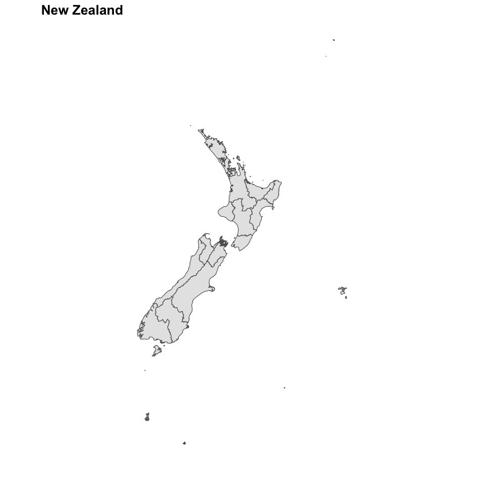
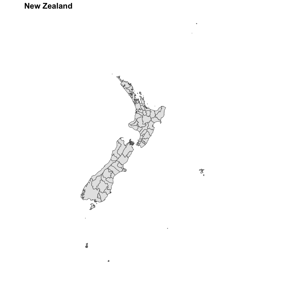
another one to extract relevant information (administrative units of level 1 to 3),
and a third one to load the data in R.
The first function, download_map():
#' Download GADM shapefile (version 4.1)#' #' @param country_name name of the country#' @param country_code ISO-3 country code#' @param country_name_clear name of the country withour space or \'download_map <-function(country_name, country_code, country_name_clear) { file_name <-str_c("gadm41_", country_code, "_shp.zip") url <-str_c("https://geodata.ucdavis.edu/gadm/gadm4.1/shp/", file_name) dest_file <-str_c("../data/Maps/GADM-4.1/", str_replace_all(country_name_clear, " ", "-"), "/", file_name )download.file(url = url, destfile = dest_file)}
And the second one, import_map() which imports the maps data from the shapefile, extracts the 3 layers corresponding to administrative units (if available) and then saves them in the country’s directory.
#' Imports map data downloaded from GADM, extracts layers and saves the result#' #' @param country_name name of the country#' @param country_code ISO-3 country code#' @param country_name_clear name of the country withour space or \'#' #' @returns the `NULL` objectimport_map <-function(country_name, country_code, country_name_clear) { out_directory <-tempfile() dir <-"../data/Maps/GADM-4.1/" file <-str_c(dir, country_name_clear, "/gadm41_", country_code, "_shp.zip") layer_0 <-str_c("gadm41_", country_code, "_0") layer_1 <-str_c("gadm41_", country_code, "_1") layer_2 <-str_c("gadm41_", country_code, "_2")unzip(file, exdir = out_directory) map_level_0 <-st_read(dsn = out_directory, layer = layer_0, quiet =TRUE) map_level_1 <-st_read(dsn = out_directory, layer = layer_1, quiet =TRUE) map_level_2 <-try(st_read(dsn = out_directory, layer = layer_2, quiet =TRUE))if (inherits(map_level_2, "try-error")) map_level_2 <-NULL res <-list(map_level_0 = map_level_0,map_level_1 = map_level_1,map_level_2 = map_level_2 ) res_name <-str_to_lower(str_c(country_code, "_maps"))assign(res_name, res)eval(parse(text =paste0("save('", res_name,"', file = '", dir, "/", country_name_clear, "/", res_name, ".RData')") ))NULL}
#' Load the layers of a country's map#' #' @param country_name name of the country#' @param tb_countries tibble with the names of countries (`country_code`),#' the corresponding ISO-3 classification (`country_code`)load_country_map <-function(country_name, tb_countries) { current_tb_country <- tb_countries |>filter(country_name ==!!country_name) country_code <- current_tb_country$country_code country_name_clear <- current_tb_country$country_name_clear current_folder <-str_c("../data/Maps/GADM-4.1/", country_name_clear) output_name <-str_c( current_folder, "/",str_to_lower(str_c(country_code, "_maps")),".RData" )load(output_name) object_name <-str_c(str_to_lower(country_code), "_maps")get(object_name)}
2.2 Download Data
Let us loop over the countries (just New Zealand here) to download the shapefiles.
cli::cli_progress_bar("Downloading SHP files", total =nrow(tb_countries))for (i in1:nrow(tb_countries)) { current_country_name <- tb_countries$country_name[i] current_country_code <- tb_countries$country_code[i] current_country_name_clear <- tb_countries$country_name_clear[i] current_folder <-str_c("../data/Maps/GADM-4.1/", current_country_name_clear)# If data not already downloaded:# Create folder and download dataif (!dir.exists(current_folder)) {dir.create(current_folder, recursive =TRUE)download_map(country_name = current_country_name,country_code = current_country_code,country_name_clear = current_country_name_clear ) } cli::cli_progress_update()}cli::cli_progress_done()
2.3 Import Shapefiles
Now that the shapefiles were downloaded, we can extract the information from them and save the extracted information into RData files that can be loaded when needed.
Let us loop again on the countries. We can do it in a parallel way, to fasten the process.
library(future)nb_cores <- future::availableCores()-1plan(multisession, workers = nb_cores)progressr::with_progress({ p <- progressr::progressor(steps =nrow(tb_countries)) tmp <- furrr::future_map(.x =1:nrow(tb_countries),#looping on the row numbers.f =~{ current_country_name <- tb_countries$country_name[.x] current_country_code <- tb_countries$country_code[.x] current_country_name_clear <- tb_countries$country_name_clear[.x]# Check if the file already exists current_folder <-str_c("../data/Maps/GADM-4.1/", current_country_name_clear) output_name <-str_c( current_folder, "/",str_to_lower(str_c(current_country_code, "_maps")),".RData" )if (!file.exists(output_name)) {# If it does not# Import the data and save the extracted informationimport_map(country_name = tb_countries$country_name[.x],country_code = tb_countries$country_code[.x],country_name_clear = tb_countries$country_name_clear[.x] ) }p()NULL } )})
2.4 Load Extracted Maps
All the maps of interest for the study have been downloaded and the information we are looking for has been extracted. We can easily load the data now. Let us create a list with all the maps from all the countries of interest.
The borders are too precise for what we need to do. Let us simplify the objects (this will allow us to have lighter graph files without loosing too much detail).
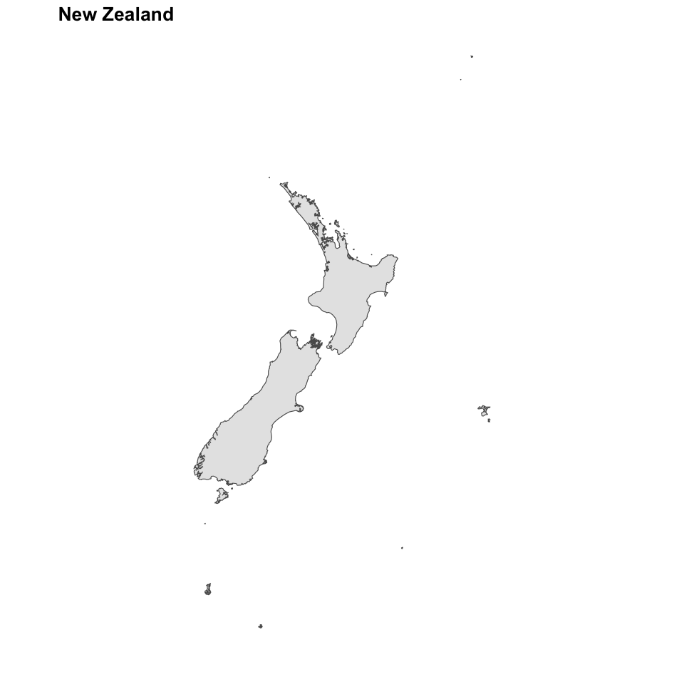
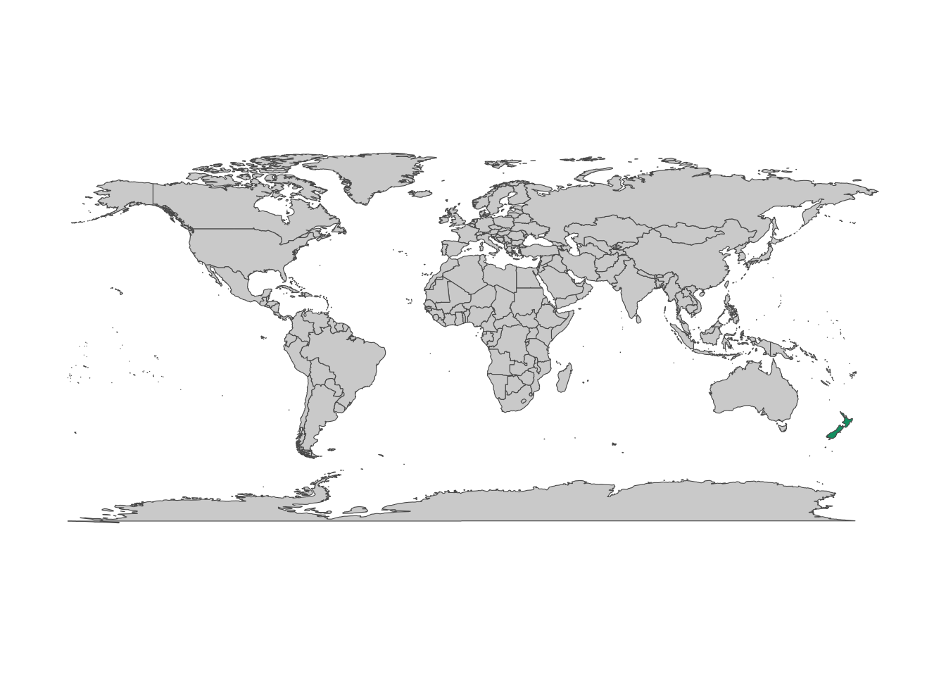
2.4.1 Level 0 (borders)
Level 0 maps corresponds to the countries boundaries.
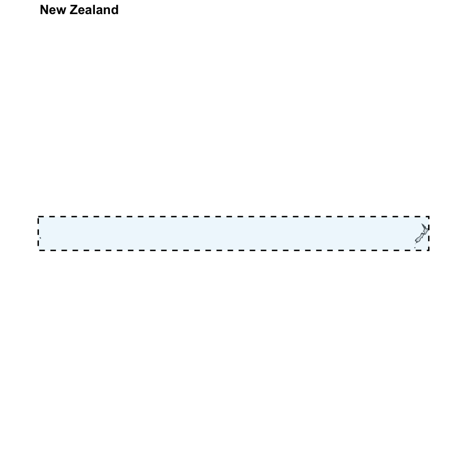
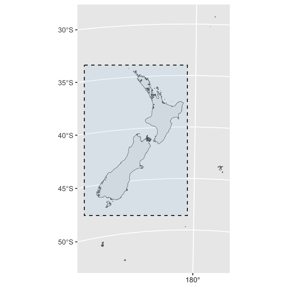
When we download gridded weather data, we will focus on the parts of the grid that correspond to New Zealand. Let us get the bounding box of the country to make this task easier. We show the R code to do so here, but we will evaluate it again in [Chapter @-sec-weather-data].
bboxes <-map(maps_level_0, st_bbox)
Note
If you re-use this code for the Fiji Islands or New Zealand, be careful. The bounding box needs to be recreated. Otherwise, it is too large, as the coordinates of this country is not convenient to work with using this map projection.