6 Background on Phenomenological Models

This chapter provides a bit of background about phenomenological models that can be used to model an epidemic.

6.1 Simple phenomenological models

We will present three models to estimate the number of cases and the number of deaths: the logistic model, the Gompertz model, and the Richards model.

6.1.1 A Generic Equation

Wang, Wu, and Yang (2012) develop the similarity between the SIR model and the Richards population model Richards (1959) which lead them to consider the following growth equation for confirmed cases noted $C (t)$ : $\begin{matrix} (6.1) & \frac{d C}{d t} = r C^{α} [1 - {(\frac{C}{K})}^{δ}], \end{matrix}$ with $r$ , $α$ , $δ$ and $K$ being positive real numbers with the further restriction $0 \leq α \leq 1$ .

A general solution to this equation has the form: $C (t) = F (r, α, δ, K, t),$ with the property that $lim_{t \to \infty} C (t) = K$ . If $C (t)$ corresponds to the total number of cases, the number of new cases is found by computing the derivative of $C (t)$ with respect to $t$ and noted $c (t)$ . The relative speed of the process is defined as $c (t) / C (t)$ and is constant over time only when $α = 1$ , $δ = 0$ . The doubling time is constant over time only under those restrictions.

A crucial question is to characterize the speed at which the process will reach its peak and when. Tsoularis and Wallace (2002) have shown that the value of the peak is given by the value of $C$ at the inflexion point of the curve: $\begin{matrix} (6.2) & C_{i n f} = K {(1 + \frac{δ}{α})}^{- 1 / δ} . \end{matrix}$ The corresponding time, that we shall note $τ$ is obtained by inverting $C (t)$ . For some models, when an analytical expression for $C (t)$ is available, $τ$ can be directly included in the parameterization. This point is of particular importance because it corresponds to the period when the epidemic starts to regress, or equivalently when the effective reproduction number $R_{t}$ starts to be below 1.

6.1.2 Logistic Model

The logistic model initiated by Verhulst (1845) provides the most simple solution to the Equation 6.1 and corresponds to $α = δ = 1$ : $\begin{matrix} (6.3) & C (t) = \frac{K}{1 + \exp (- r (t - τ))} . \end{matrix}$

It has been recently applied to study the evolution of an epidemic Ma (2020). We have introduced a parameterization where $τ$ directly represents the inflection point with that $C (τ) = K / 2$ . So the peak is at the mid of the epidemic which reaches its cumulated maximum $K$ , $r$ representing the growth rate. The first order derivative of this function provides an estimate of the number of cases at each point in time: $\frac{\partial C (t)}{\partial t} = \frac{K r \exp (- r (t - τ))}{{[1 + \exp (- r (t - τ)]}^{2}} .$ The relative speed is thus: $\frac{c (t)}{C (t)} = r \frac{e^{- r (t - τ)}}{1 + e^{- r (t - τ)}} .$ This model might appear as a nice solution to represents the three phases of an epidemic, but we shall discover below that its symmetry tends to be in contradiction with epidemic data. So we have to explore alternative solutions.

In R, we define the logistic function as follows:

#' Logistic function
#' 
#' @param theta vector of named parameters
#' @param x time
logistic_f <-  function(theta, x) {
  k <- theta[["k"]]
  tau <- theta[["tau"]]
  r <- theta[["r"]]
  k / ( 1+exp( -r*( x - tau ) ) )
}

#' First derivative of the logistic function
#' 
#' @param theta vector of named parameters
#' @param x time
logistic_f_first_d <- function(theta, x) {
  k <- theta[["k"]]
  tau <- theta[["tau"]]
  r <- theta[["r"]]
  
  (k * r * exp( -r * (x - tau) )) / (1+ exp( -r * (x - tau) ))^2
}

#' Second derivative of the logistic function
#' 
#' @param theta vector of named parameters
#' @param x time
logistic_f_second_d <- function(theta, x) {
  k <- theta[["k"]]
  tau <- theta[["tau"]]
  r <- theta[["r"]]
  
  k*((2*r^2 * exp(-2*r*(x - tau)))/
       (exp(-r*(x - tau)) + 1)^3 - 
       (r^2*exp(-r*(x - tau)))/(exp(-r*(x - tau)) + 1)^2)
}

Now, let us make some graph to give an idea of how the dynamic changes with the parameters $r$ and $t a u$ .

library(tidyverse)

── Attaching core tidyverse packages ──────────────────────── tidyverse 2.0.0 ──
✔ dplyr     1.1.2     ✔ readr     2.1.4
✔ forcats   1.0.0     ✔ stringr   1.5.0
✔ ggplot2   3.4.2     ✔ tibble    3.2.1
✔ lubridate 1.9.2     ✔ tidyr     1.3.0
✔ purrr     1.0.1     
── Conflicts ────────────────────────────────────────── tidyverse_conflicts() ──
✖ dplyr::filter() masks stats::filter()
✖ dplyr::lag()    masks stats::lag()
ℹ Use the conflicted package (<http://conflicted.r-lib.org/>) to force all conflicts to become errors

library(scales)


Attaching package: 'scales'

The following object is masked from 'package:purrr':

    discard

The following object is masked from 'package:readr':

    col_factor

g_legend<-function(a.gplot){
  tmp <- ggplot_gtable(ggplot_build(a.gplot))
  leg <- which(sapply(tmp$grobs, function(x) x$name) == "guide-box")
  legend <- tmp$grobs[[leg]]
  return(legend)}

The different values for $r$ and $t a u$ ( $k$ is set to 5000).

situations <- 
  expand_grid(tau = c(25,35), r = c(.15, .25, .35)) |> 
  mutate(k = 5000)

Let us apply, for a set of parameters, at different time horizon (from 0 to 60 by steps of .1) the logistic function, its first and second derivatives with respect to time. To do so, we define a “simulation” function:

#' Simulation of the logistic model for some parameters
#' 
#' @param i row number of situations
simu <- function(i) {
  current_params <- situations |> slice(i)
  current_params <- c(as_vector(current_params)) |> as.list()
  
  n     <- 60
  step  <- .01
  sim   <-  logistic_f(
    theta = current_params, 
    x = seq(0,n, by = step)
  )
  simD  <-  logistic_f_first_d(
    theta = current_params, 
    x = seq(0,n, by = step)
  )
  simD2 <-  logistic_f_second_d(
    theta = current_params, 
    x = seq(0,n, by = step)
  )
  
  tibble(
    t = seq(0, n, by = step),
    k = current_params[["k"]], 
    tau = current_params[["tau"]],
    r = current_params[["r"]],
    sim = sim
  ) |> 
    mutate(
      simD = simD,
      simD2 = simD2
    )
}

Let us do so for all the different sets of parameters:

simu_res <- map_df(1:nrow(situations), simu)

We would like to show the thresholds on the graph:

threshold_times <- 
  simu_res |> 
  group_by(k, tau, r) |> 
  summarise(threshold_time = unique(tau)) |> 
  ungroup() |> 
  mutate(
    r = str_c("$\\r = ", r, "$"),
    tau = str_c("$\\tau = ", tau, "$")
  )

`summarise()` has grouped output by 'k', 'tau'. You can override using the
`.groups` argument.

threshold_times

# A tibble: 6 × 4
      k tau            r              threshold_time
  <dbl> <chr>          <chr>                   <dbl>
1  5000 "$\\tau = 25$" "$\\r = 0.15$"             25
2  5000 "$\\tau = 25$" "$\\r = 0.25$"             25
3  5000 "$\\tau = 25$" "$\\r = 0.35$"             25
4  5000 "$\\tau = 35$" "$\\r = 0.15$"             35
5  5000 "$\\tau = 35$" "$\\r = 0.25$"             35
6  5000 "$\\tau = 35$" "$\\r = 0.35$"             35

Now, we are ready to create the plots:

p_simu_logis <- 
  ggplot(
    data =  simu_res |> 
      mutate(
        r = str_c("$\\r = ", r, "$"),
        tau = str_c("$\\tau = ", tau, "$")
      ),
    mapping = aes(x = t)
  ) +
  geom_line(mapping = aes(y = sim, linetype = "sim")) +
  geom_line(mapping = aes(y = simD*10, linetype = "simD")) +
  geom_line(mapping = aes(y = simD2*10, linetype = "simD2")) +
  geom_vline(
    data = threshold_times, 
    mapping = aes(xintercept = threshold_time),
    colour = "red", linetype = "dotted") +
  facet_grid(
    r~tau, 
    labeller = as_labeller(
      latex2exp::TeX, 
      default = label_parsed
    )
  ) +
  labs(x = "Time", y = latex2exp::TeX("$F(t)$")) +
  scale_y_continuous(
    labels = scales::comma,
    sec.axis = sec_axis(
      ~./10, 
      name = latex2exp::TeX(
        "$\\partial F(t) / \\partial t$, $\\partial^2 F(t) / \\partial t^2$"
      ),
      labels = comma)) +
  scale_linetype_manual(
    NULL,
    values = c("sim" = "solid", "simD" = "dashed", "simD2" = "dotdash"),
    labels = c(
      "sim" = latex2exp::TeX("$F(t)$"), 
      "simD" = latex2exp::TeX("$\\partial F(t) / \\partial t$"),
      "simD2" = latex2exp::TeX("$\\partial^2 F(t) / \\partial t^2$"))) +
  theme(axis.ticks.y = element_blank())

p_simu_logis +
  theme_minimal() +
  theme(legend.position = "bottom")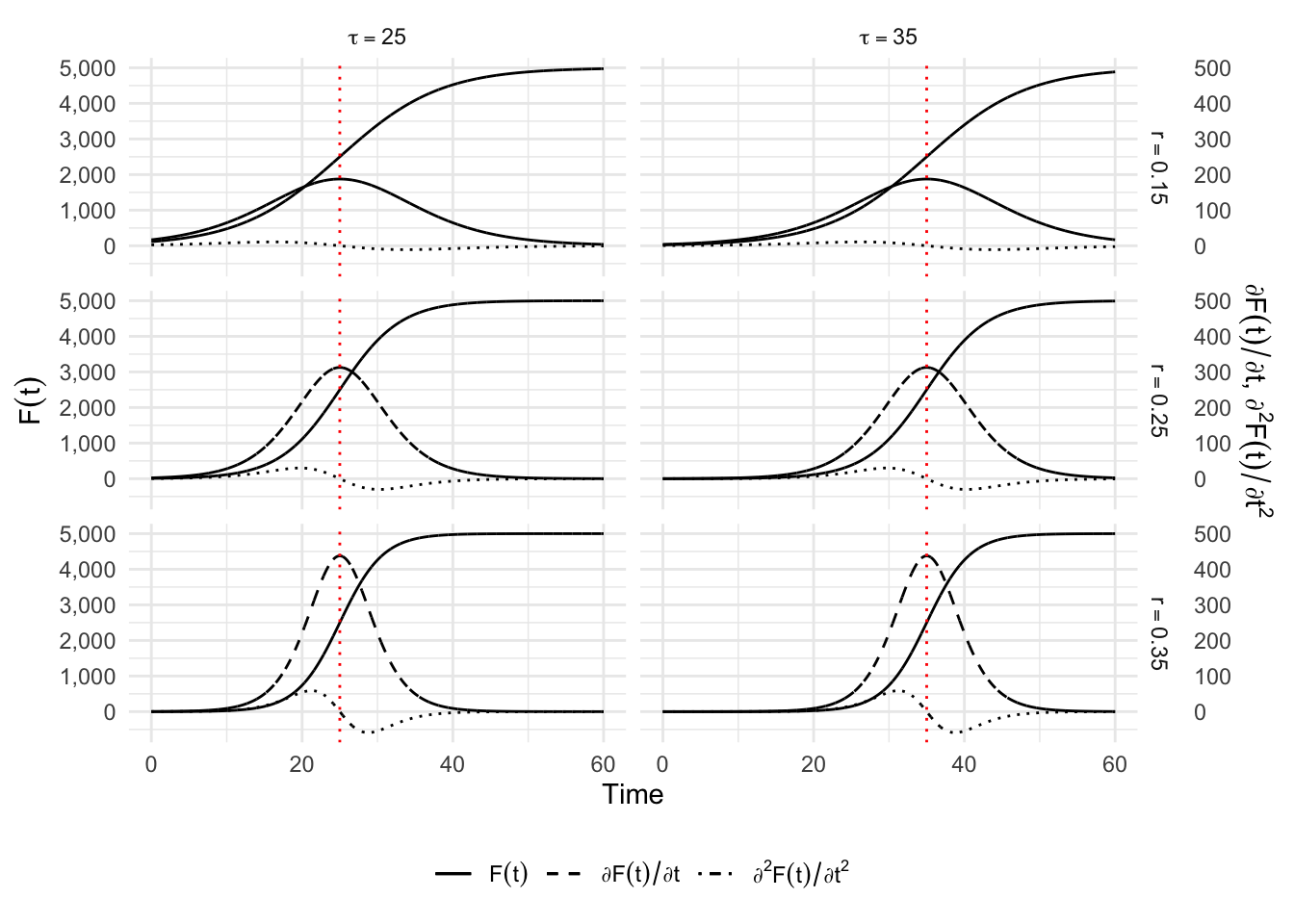

Figure 6.1: Illustration of the logistic model for different values for $τ$ and $r$ , with $k = 5, 000$

6.1.2.1 Key moments

Let us focus on the key moment of the epidemics. Let us illustrate them using one of the scenarios.

data_sim <- simu(1)

The starting point:

df_starting <- 
  data_sim %>% 
  filter(sim >= 1) %>% 
  slice(1)

The acceleration point

df_acceleration <- 
  data_sim %>% 
  filter(simD2 == max(simD2)) %>% 
  slice(1)

The peak:

df_peak <- 
  data_sim %>% 
  filter(simD == max(simD)) %>% 
  slice(1)

The deceleration point:

df_deceleration <- 
  data_sim %>% 
  filter(simD2 == min(simD2)) %>% 
  slice(1)

The return point:

df_return <- 
  data_sim %>% 
  filter(sim > k - 1) %>% 
  slice(1)

Let us reshape the data:

df_plot_key_moments <- 
  data_sim %>% 
  gather(key, value, sim, simD, simD2)

df_plot_key_moments_points <- 
  df_acceleration %>% mutate(label = "$t_A$") %>% 
  bind_rows(df_peak %>% mutate(label = "$t_P$")) %>% 
  bind_rows(df_deceleration %>% mutate(label = "$t_D$"))

And the plot:

p_key_moments <- 
  ggplot() +
  geom_hline(yintercept = 0, col = "grey") +
  geom_line(
    data = df_plot_key_moments,
    mapping = aes(x = t, y = value, linetype = key)
  ) +
  geom_segment(
    data = df_plot_key_moments_points,
    mapping = aes(x = t, xend = t, y = 0, yend = sim),
    linetype = "dotted", colour = "red"
  ) +
  geom_point(
    data = df_plot_key_moments_points,
    mapping = aes(x = t, y = sim), size = 2
  ) +
  geom_point(
    data = df_plot_key_moments_points,
    mapping = aes(x = t, y = sim),
    size = 1, colour = "white"
    ) +
  geom_text(
    data = df_plot_key_moments_points,
    mapping = aes(x = t-2, y = sim + .05*k, label = label)
  ) +
  labs(x = "Time", y = latex2exp::TeX("$F(t)$")) +
  scale_linetype_manual(
    NULL,
    values = c("sim" = "solid", "simD" = "dashed", "simD2" = "dotdash"),
    labels = c(
      "sim" = latex2exp::TeX("$F(t)$"),
      "simD" = latex2exp::TeX("$\\partial F(t) / \\partial t$"),
      "simD2" = latex2exp::TeX("$\\partial^2 F(t) / \\partial t^2$")
    )
  ) +
  theme(axis.text = element_blank(), axis.ticks = element_blank())

p_key_moments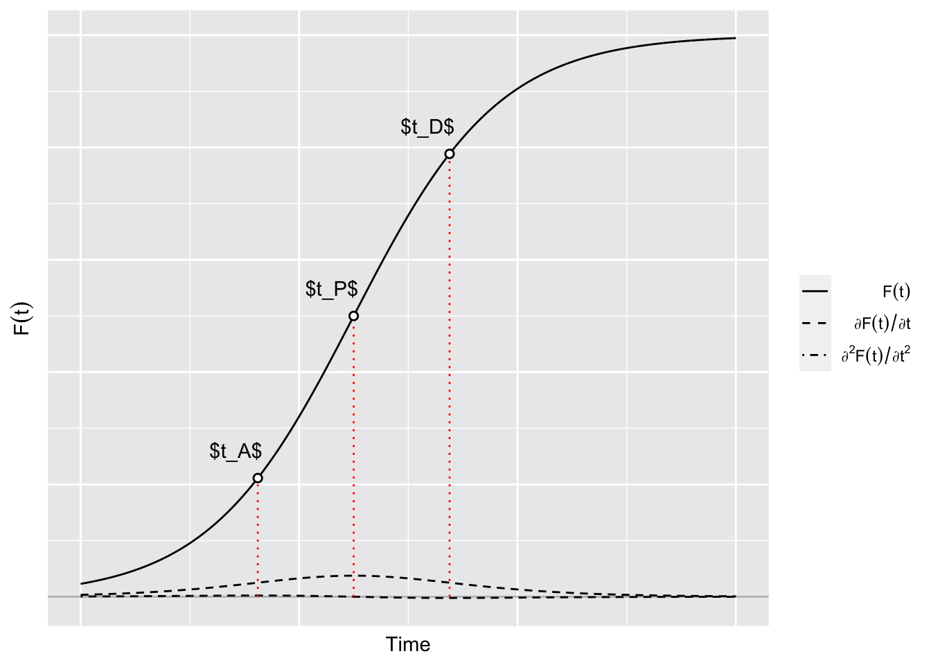

Figure 6.2: Key moments of the epidemics, using a logistim model.

6.1.3 Gompertz Model

The Gompertz model (Gompertz 1825) has three parameters, but corresponds to alternative restrictions with $α = 1$ but this time $δ = 0$ . The solution to Equation 6.1 can be written as follows Tjørve and Tjørve (2017): $\begin{matrix} (6.4) & C (t) = K \exp [- \exp (- r (t - τ))] . \end{matrix}$ In Equation 6.4, the parameters are interpreted in the same way as those of the logistic model. The main difference between the logistic and Gompertz models is that the latter is not symmetric around the inflection point, which now appears earlier as $C (τ) = K / e$ . The first order derivative of this function provides an estimate of the number of cases at each point in time: $\frac{\partial C (t)}{\partial t} = K r \exp [r (τ - t) - \exp (r (τ - t))] .$ So that the relative speed of the epidemic is given by: $\frac{c (t)}{C (t)} = r e^{- r (t - τ)},$ with of course a maximum speed at the peak.

In R, this translates to:

#' Gompertz function with three parameters
#' 
#' @param theta vector of named parameters
#' @param x time
gompertz_f <- function(theta, x) {
  k <- theta[["k"]]
  tau <- theta[["tau"]]
  r <- theta[["r"]]
  k*exp( -exp( -r * (x - tau) ) )
}
#' First order derivative of Gompertz wrt x
#' 
#' @param theta vector of named parameters
#' @param x time
gompertz_f_first_d <- function(theta, x) {
  k <- theta[["k"]]
  tau <- theta[["tau"]]
  r <- theta[["r"]]
  
  k * (x - tau) * exp(r * (tau - x) - exp(r * (tau - x)))
}

#' Second order derivative of Gompertz
#' 
#' @param theta vector of named parameters
#' @param x time
gompertz_f_second_d <- function(theta, x) {
  k <- theta[["k"]]
  tau <- theta[["tau"]]
  r <- theta[["r"]]
  
  -k * r^2 * exp(-r * (x - tau)) * 
    exp(-exp(-r * (x - tau))) + 
    k * r^2 * (exp(-r * (x - tau)))^2 * exp(-exp(-r * (x - tau)))
}

Let us make some graph to give an idea of how the dynamic changes with the parameters $r$ and $t a u$ .

k <- 5000
situations <- 
  expand_grid(tau = c(25,35), r = c(.15, .25, .35)) |> 
  mutate(k = k)

#' Simulation of the logistic model for some parameters
#' 
#' @param i row number of situations
simu_gomp <- function(i) {
  current_params <- situations |> slice(i)
  current_params <- c(as_vector(current_params)) |> as.list()
  
  n <- 60
  step <- .01
  sim <-  gompertz_f(theta = current_params, x = seq(1,n, by = step))
  simD <-  gompertz_f_first_d(theta = current_params, x = seq(1,n, by = step))
  simD2 <-  gompertz_f_second_d(theta = current_params, x = seq(1,n, by = step))
  
  tibble(
    t = seq(1, n, by = step),
    k = current_params[["k"]],
    tau = current_params[["tau"]],
    r = current_params[["r"]],
    sim = sim) |> 
    mutate(simD = simD,
           simD2 = simD2)
  
}

The values of $C (t)$ , its first and second derivatives with respect to time can be computed for the different scenarios:

simu_gomp_res <- map_df(1:nrow(situations), simu_gomp)

The threshold for each scenario:

threshold_times <-
  simu_gomp_res |>
  group_by(k, tau, r) |>
  summarise(threshold_time = unique(tau)) |>
  ungroup() |> 
  mutate(
    r = str_c("$\\r = ", r, "$"),
    tau = str_c("$\\tau = ", tau, "$")
  )

`summarise()` has grouped output by 'k', 'tau'. You can override using the
`.groups` argument.

And we can plot the results:

p_simu_gomp <- 
  ggplot(
  data = simu_gomp_res |> 
    mutate(
      r = str_c("$\\r = ", r, "$"),
      tau = str_c("$\\tau = ", tau, "$")
    ),
  mapping = aes(x = t)) +
  geom_line(mapping = aes(y = sim, linetype = "sim")) +
  geom_line(mapping = aes(y = simD, linetype = "simD")) +
  geom_line(mapping = aes(y = simD2, linetype = "simD2")) +
  facet_grid(
    r~tau,
    labeller = as_labeller(
      latex2exp::TeX, 
      default = label_parsed
    )
  ) +
  geom_vline(
    data = threshold_times, 
    mapping = aes(xintercept = threshold_time), 
    colour = "red", linetype = "dotted") +
  labs(x = "Time", y = latex2exp::TeX("$F(t)$")) +
  scale_linetype_manual(
    NULL,
    values = c("sim" = "solid", "simD" = "dashed", "simD2" = "dotdash"),
    labels = c("sim" = latex2exp::TeX("$F(t)$"),
               "simD" = latex2exp::TeX("$\\partial F(t) / \\partial t$"),
               "simD2" = latex2exp::TeX("$\\partial^2 F(t) / \\partial t^2$")
    )
  ) +
  theme(axis.ticks.y = element_blank())

p_simu_gomp +
  theme_minimal() +
  theme(legend.position = "bottom")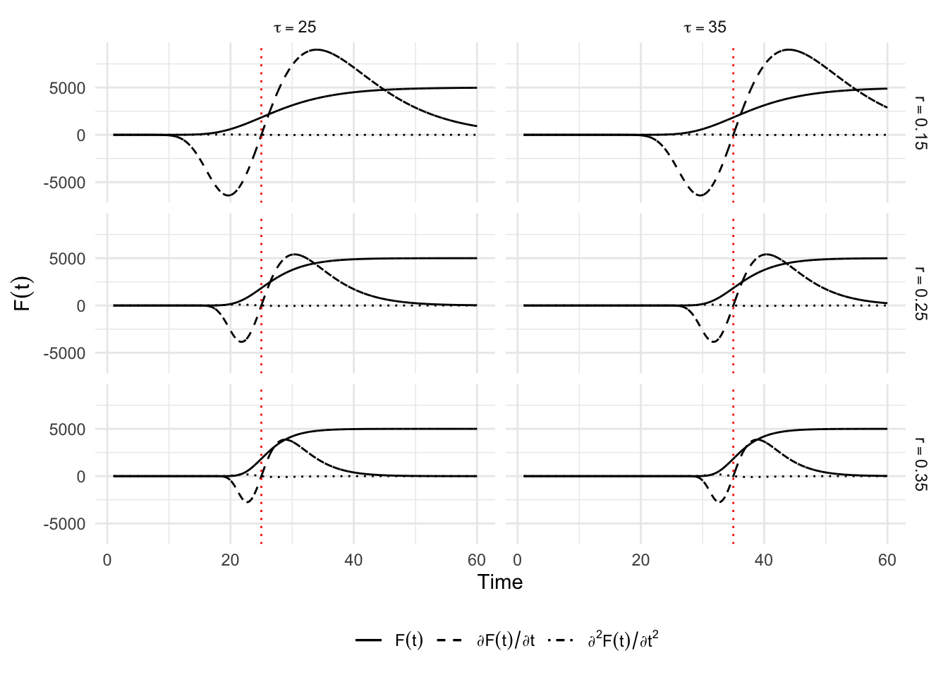

Figure 6.3: Illustration of Gompertz model for different values for $τ$ and $r$ , with $k = 5, 000$

6.1.4 Richards Model

The question “what happens with $0 < δ < 1$ ” finds an answer with Richards (1959) and the Richards model which is widely used in nonlinear regression analysis. The solution to Equation 6.1 provided in Lee, Lei, and Mallick (2020) corresponds to: $C (t) = K {[1 + δ \exp (- r (t - τ))]}^{- 1 / δ},$ where parameters $K$ and $τ$ and are interpreted in the same way as those of the logistic and Gompertz models, while the growth rate is now $r / δ$ . The parameter $δ > 0$ is used to control the value of the curve at the inflection point $C (τ) = K / (1 + δ)^{1 / δ}$ , and thus the asymmetry around $t = τ$ . This model considers one more parameter than the Gompertz model to model this asymmetry. The first order derivative of this function will provide an estimate of the number of cases at each point in time: $\frac{\partial C (t)}{\partial t} = \frac{K r {[δ \exp (r (τ - t)) + 1]}^{- 1 / δ}}{δ + \exp (r (t - τ))},$ leading to a relative speed of: $\frac{c (t)}{C (t)} = r \frac{e^{- r (t - τ)}}{1 + δ e^{- r (t - τ)}} .$ This model is also a generalization of the two previous ones as can be seen for instance when comparing the different relative speeds.

In R, this translates to the following functions:

#' Richards function with four parameters
#' 
#' @param theta vector of named parameters
#' @param x time
richards_f <- function(theta, x) {
  k <- theta[["k"]]
  tau <- theta[["tau"]]
  r <- theta[["r"]]
  delta <- theta[["delta"]]
  
  k / (1 + delta * exp(-r * delta * (x - tau)))^(1 / delta)
}


#' First order derivative of Richards function wrt time (x)
#' 
#' @param theta vector of named parameters
#' @param x time
richards_f_first_d <- function(theta, x) {
  k <- theta[["k"]]
  tau <- theta[["tau"]]
  r <- theta[["r"]]
  delta <- theta[["delta"]]
  
  delta * k * r * exp(delta * (-r) * (x - tau)) * 
    (delta * exp(delta * (-r) * (x - tau)) + 1)^(-1 / delta - 1)
}


#' Second order derivative of Richards function wrt time (x)
#' 
#' @param theta vector of named parameters
#' @param x time
richards_f_second_d <- function(theta, x) {
  k <- theta[["k"]]
  tau <- theta[["tau"]]
  r <- theta[["r"]]
  delta <- theta[["delta"]]
  
  k * ((-1 / delta - 1) * 
         delta^3 * r^2 * (-exp(-2 * delta * r * (x - tau))) *
         (delta * exp(delta * (-r) * (x - tau)) + 1)^(-1 / delta - 2) - 
         delta^2 * r^2 * exp(delta * (-r) * (x - tau)) * 
         (delta * exp(delta * (-r) * (x - tau)) + 1)^(-1 / delta - 1))
}

Again, let us provide different scenarios to plot the curves for $C (t)$ , its first and second derivatives with respect to time. We will make the parameters $δ$ and $r$ vary. We set $k$ to $5, 000$ and $τ$ to 25.

situations <- 
  expand_grid(delta = c(.5, 1.5), r = c(.15, .25, .35)) |> 
  mutate(k = 5000, tau = 25)

We create a function to get the values of $C (t)$ and its derivatives depending on the scenario.

#' Simulation of Richards model for some parameters
#' 
#' @param i row number of situations
simu_richards <- function(i) {
  current_params <- situations |> slice(i)
  current_params <- c(as_vector(current_params)) |> as.list()
  
  n <- 60
  step <- .01
  sim <-  richards_f(theta = current_params, x = seq(1,n, by = step))
  simD <-  richards_f_first_d(theta = current_params, x = seq(1,n, by = step))
  simD2 <-  richards_f_second_d(theta = current_params, x = seq(1,n, by = step))
  
  tibble(
    t = seq(1, n, by = step),
    k = current_params[["k"]], 
    tau = current_params[["tau"]],
    r = current_params[["r"]],
    delta = current_params[["delta"]],
    sim = sim
    ) |> 
    mutate(simD = simD,
           simD2 = simD2)
}

This function is then applied to the different scenarios:

simu_richards_res <- map_df(1:nrow(situations), simu_richards)

The thresholds:

threshold_times <-
  simu_richards_res |>
  group_by(k, tau, r, delta) |>
  summarise(threshold_time = unique(tau)) |>
  ungroup() |>
  mutate(
    r = str_c("$r = ", r, "$"),
    delta = str_c("$\\delta = ", delta, "$")
  )

`summarise()` has grouped output by 'k', 'tau', 'r'. You can override using the
`.groups` argument.

p_simu_richards <- 
  ggplot(
    data = simu_richards_res |> 
      mutate(
        r = str_c("$r = ", r, "$"),
        delta = str_c("$\\delta = ", delta, "$")
      ),
    mapping = aes(x = t)
  ) +
  geom_line(mapping = aes(y = sim, linetype = "sim")) +
  geom_line(mapping = aes(y = simD * 10, linetype = "simD")) +
  geom_line(mapping = aes(y = simD2 * 10, linetype = "simD2")) +
  facet_grid(
    r ~ delta,
    labeller = as_labeller(
      latex2exp::TeX, 
      default = label_parsed
    )
  ) +
  geom_vline(
    data = threshold_times, 
    mapping = aes(xintercept = threshold_time),
    colour = "red", linetype = "dotted") +
  labs(x = "Time", y = latex2exp::TeX("$F(t)$")) +
  scale_y_continuous(
    labels = comma,
    breaks = seq(0, 5000, by = 1000),
    sec.axis = sec_axis(
      ~./10,
      name = latex2exp::TeX(
        "$\\partial F(t)/\\partial t$, $\\partial^2 F(t)/\\partial t^2$"
      ),
      labels = comma)
  ) +
  scale_linetype_manual(
    NULL,
    values = c("sim" = "solid", "simD" = "dashed", "simD2" = "dotdash"),
    labels = c("sim" = latex2exp::TeX("$F(t)$"),
               "simD" = latex2exp::TeX("$\\partial F(t) / \\partial t$"),
               "simD2" = latex2exp::TeX("$\\partial^2 F(t) / \\partial t^2$"))
  ) +
  theme(axis.ticks.y = element_blank())

p_simu_richards +
  theme_minimal() +
  theme(legend.position = "bottom")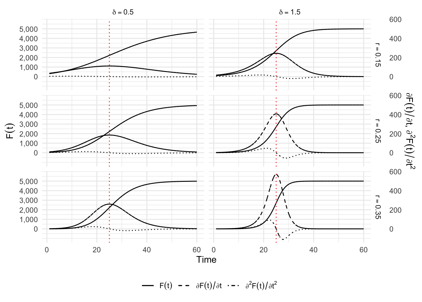

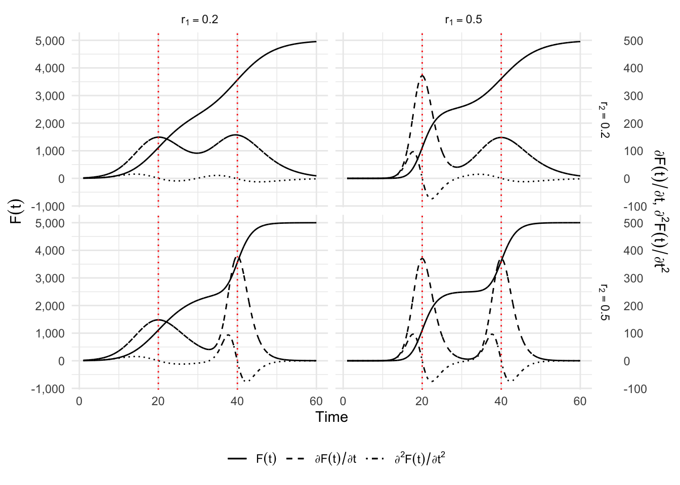
Figure 6.4: Illustration of Richards’ model for different values for $δ$ and $r$ , with $k = 5, 000$ and $τ = 25$

6.2 Double sigmoid functions to account for a second wave

One possibility to account for two distinct phases is to use a double sigmoid. This is done by adding or multiplying two sigmoid functions, as follows: $C (t) = C_{1}^{(m_{1})} (t) + C_{2}^{(m_{2})} (t),$ where $C_{1}^{(m_{1})} (t)$ is the first sigmoid function and $C_{2}^{(m_{2})} (t)$ is the second one. The types $m_{1}$ and $m_{2}$ of sigmoid can be, for example, a logistic curve (see, e.g., Lipovetsky (2010) or Bock et al. (1973)), a Gompertz curve Thissen et al. (1976), or a Richards curve Oswald et al. (2012).

We limit ourselves here to the presentation of a double-Gompertz curve: $\begin{aligned} C (t) = & K_{1} \exp [- \exp (- r_{1} (t - τ_{1}))] \\ + (K_{2} - K_{1}) \exp [- \exp (- r_{2} (t - τ_{2}))], \end{aligned}$ where $K_{1}$ and $K_{2}$ are the intermediate and final plateau of saturation, respectively. The parameters $τ_{1}$ and $τ_{2}$ define the inflection points of each phase when the intermediate plateau is long enough while the growth of the process is determined by $r_{1}$ and $r_{2}$ , for the first and second sigmoid. However there is no analytical formula to determine the value and position of the two peaks. We have to evaluate numerically the extremum of the second order derivative of $C (t)$ . The first order derivative of $C (t)$ provides an estimate of the number of cases at each point of time: $\begin{aligned} \frac{\partial C (t)}{\partial t} = & K_{1} r_{1} \exp (- r_{1} (t - τ_{1}) \exp (- \exp (- r 1 (t - τ 1))) \\ + (K_{2} - K_{1}) r_{2} \exp (- r_{2} (t - τ_{2}) \exp (- \exp (- r 2 (t - τ 2))) . \end{aligned}$ The formula giving the relative speed $c (t) / C (t)$ does not lead to any simplification and will not be detailed.

6.2.1 Double Logistic

The double logistic function, its first and second derivatives with respect to time can be coded as follows:

# Double logistic
double_logistic_f <-  function(theta, x) {
  K1 <- theta[["K1"]]
  tau1 <- theta[["tau1"]]
  r1 <- theta[["r1"]]
  K2 <- theta[["K2"]]
  tau2 <- theta[["tau2"]]
  r2 <- theta[["r2"]]
  
  (K1/(1 + exp(-r1 * (x - tau1)))) + ((K2 - K1)/(1 + exp(-r2 * (x - tau2))))
}
# Double logistic in two parts
double_logistic_f_2 <- function(theta, x) {
  K1 <- theta[["K1"]]
  tau1 <- theta[["tau1"]]
  r1 <- theta[["r1"]]
  K2 <- theta[["K2"]]
  tau2 <- theta[["tau2"]]
  r2 <- theta[["r2"]]
  
  f_1 <- K1 / (1 + exp(-r1 * (x - tau1)))
  f_2 <- (K2 - K1)/(1 + exp(-r2 * (x - tau2)))
  tibble(x = x, f_1 = f_1, f_2 = f_2)
}

# First derivative
double_logistic_f_first_d <-  function(theta, x) {
  K1 <- theta[["K1"]]
  tau1 <- theta[["tau1"]]
  r1 <- theta[["r1"]]
  K2 <- theta[["K2"]]
  tau2 <- theta[["tau2"]]
  r2 <- theta[["r2"]]
  
  (r1 * K1 * exp(-r1 * (x - tau1))) / ((exp(-r1 * (x-tau1)) + 1)^2) +
    (r2 * (K2-K1) * exp(-r2 * (x - tau2))) / ((exp(-r2 * (x-tau2)) + 1)^2)
}
# Second derivative
double_logistic_f_second_d <-  function(theta, x) {
  K1 <- theta[["K1"]]
  tau1 <- theta[["tau1"]]
  r1 <- theta[["r1"]]
  K2 <- theta[["K2"]]
  tau2 <- theta[["tau2"]]
  r2 <- theta[["r2"]]
  
  K1 *  ((2 * r1^2 * exp(-2 * r1 * (x - tau1)))/(exp(-r1 * (x - tau1)) + 1)^3 - 
           ( r1^2 * exp(- r1 * (x - tau1)))/(exp(-r1 * (x - tau1)) + 1)^2) +
    
    (K2-K1) *  
    ((2 * r2^2 * exp(-2 * r2 * (x - tau2)))/(exp(-r2 * (x - tau2)) + 1)^3 - 
       ( r2^2 * exp(- r2 * (x - tau2)))/(exp(-r2 * (x - tau2)) + 1)^2)
  
}

And now, let us make some illustrations by varying $r_{1}$ and $r_{2}$ .

situations <- 
  expand_grid(r1 = c(.2, .5), r2 = c(.2, .5)) |> 
  mutate(
    K1   = 2500,
    K2   = 5000,
    tau1 = 20,
    tau2 = 40
  )

The function that simulates $C (t)$ and its first and second derivatives with respect to time for a single scenario:

#' Simulation of the logistic model for some parameters
#' 
#' @param i row number of situations
simu <- function(i) {
  current_params <- situations |> slice(i)
  current_params <- c(as_vector(current_params)) |> as.list()
  
  n <- 60
  step <- .01
  sim <-  double_logistic_f(theta = current_params, x = seq(1,n, by = step))
  simD <-  double_logistic_f_first_d(
    theta = current_params, x = seq(1,n, by = step))
  simD2 <-  double_logistic_f_second_d(
    theta = current_params, x = seq(1,n, by = step))
  
  tibble(
    t = seq(1, n, by = step),
    K1 = current_params[["K1"]],
    r1 = current_params[["r1"]],
    tau1 = current_params[["tau1"]],
    K2 = current_params[["K2"]],
    r2 = current_params[["r2"]],
    tau2 = current_params[["tau2"]],
    sim = sim) |> 
    mutate(simD = simD,
           simD2 = simD2)
  
}

The simulated values for all the scenarios:

simu_res <- map_df(1:nrow(situations), simu)

The thresholds:

threshold_times <- 
  simu_res |> 
  group_by(K1, tau1, r1, K2, tau2, r2) |> 
  summarise(
    threshold_time_1 = unique(tau1),
    threshold_time_2 = unique(tau2)
  ) |> 
  ungroup() |> 
  mutate(
    r1 = str_c("$r_1 = ", r1, "$"),
    r2 = str_c("$r_2 = ", r2, "$")
  )

`summarise()` has grouped output by 'K1', 'tau1', 'r1', 'K2', 'tau2'. You can
override using the `.groups` argument.

p_simu_double_logis <- 
  ggplot(
    data = simu_res |> 
      mutate(
        r1 = str_c("$r_1 = ", r1, "$"),
        r2 = str_c("$r_2 = ", r2, "$")
      ),
    mapping = aes(x = t)
  ) +
  geom_line(aes(y = sim, linetype = "sim")) +
  geom_line(aes(y = simD * 10, linetype = "simD")) +
  geom_line(aes(y = simD2 * 10, linetype = "simD2")) +
  geom_vline(
    data = threshold_times,
    mapping = aes(xintercept = threshold_time_1),
    colour = "red", linetype = "dotted") +
  geom_vline(
    data = threshold_times,
    mapping = aes(xintercept = threshold_time_2),
    colour = "red", linetype = "dotted") +
  facet_grid(
    r2 ~ r1,
    labeller = as_labeller(
      latex2exp::TeX, 
      default = label_parsed
    )
  ) +
  labs(x = "Time", y = "$F(t)$") +
  scale_y_continuous(
    labels = comma,
    sec.axis = sec_axis(
      ~./10,
      name = latex2exp::TeX(
        "$\\partial F(t) / \\partial t$, $\\partial^2 F(t) / \\partial t^2$"
      ),
      labels = comma)
  ) +
  scale_linetype_manual(
    NULL,
    values = c("sim" = "solid", "simD" = "dashed", "simD2" = "dotdash"),
    labels = c("sim" = latex2exp::TeX("$F(t)$"), 
               "simD" = latex2exp::TeX("$\\partial F(t) / \\partial t$"),
               "simD2" = latex2exp::TeX("$\\partial^2 F(t) / \\partial t^2$"))
               ) +
  theme(axis.ticks.y = element_blank())

p_simu_double_logis +
  theme_minimal() +
  theme(legend.position = "bottom")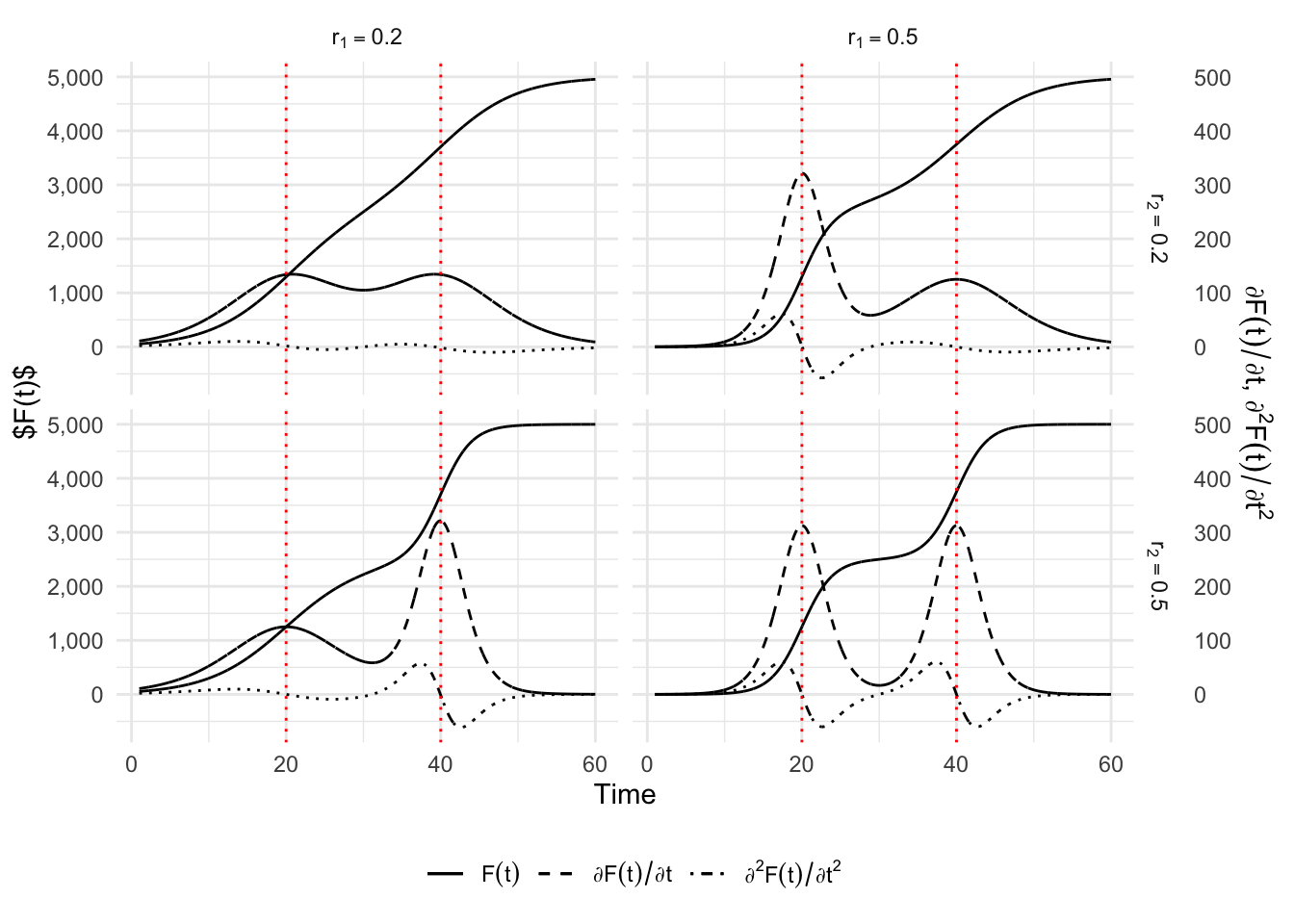

Figure 6.5: Illustration of a Double Logistic model for different values for $r_{1}$ and $r_{2}$ , with $K_{1} = 2, 500$ , $K_{2} = 5, 000$ , $τ_{1} = 20$ , and $τ_{2} = 40$

6.2.2 Double Gompertz Model

The double Gompertz function, its first and second derivatives with respect to time can be coded as follows:

# Double-Gompertz function
#' @param theta vector of named parameters
#' @param x observation / training example
double_gompertz_f <- function(theta, x) {
  K1 <- theta[["K1"]]
  tau1 <- theta[["tau1"]]
  r1 <- theta[["r1"]]
  K2 <- theta[["K2"]]
  tau2 <- theta[["tau2"]]
  r2 <- theta[["r2"]]
  
  f_1 <- K1 * exp(-exp(-r1 * (x - tau1)))
  f_2 <- (K2-K1) * exp(-exp(-r2 * (x - tau2)))
  
  f_1 + f_2
}

#' Double-Gompertz function in two parts
#' 
double_gompertz_f_2 <- function(theta, x) {
  K1 <- theta[["K1"]]
  tau1 <- theta[["tau1"]]
  r1 <- theta[["r1"]]
  K2 <- theta[["K2"]]
  tau2 <- theta[["tau2"]]
  r2 <- theta[["r2"]]

  f_1 <- K1 * exp(-exp(-r1 * (x - tau1)))
  f_2 <- (K2-K1) * exp(-exp(-r2 * (x-tau2)))
  tibble(x = x, f_1 = f_1, f_2 = f_2)
}

#' First derivative
#' 
double_gompertz_f_first_d <- function(theta, x) {
  K1 <- theta[["K1"]]
  tau1 <- theta[["tau1"]]
  r1 <- theta[["r1"]]
  K2 <- theta[["K2"]]
  tau2 <- theta[["tau2"]]
  r2 <- theta[["r2"]]

  f_1_d <- r1 * K1 * exp(-r1 * (x - tau1) - exp(- r1 * (x - tau1)))
  f_2_d <- r2 * (K2-K1) * exp(-r2 * (x - tau2) - exp(- r2 * (x - tau2)))
  
  f_1_d + f_2_d
}

#' Second derivative
double_gompertz_f_second_d <- function(theta, x) {
  K1 <- theta[["K1"]]
  tau1 <- theta[["tau1"]]
  r1 <- theta[["r1"]]
  K2 <- theta[["K2"]]
  tau2 <- theta[["tau2"]]
  r2 <- theta[["r2"]]
  
  -K1 * r1^2 * exp(-r1*(x - tau1)) * exp(-exp(-r1*(x - tau1))) +
    K1 * r1^2 * (exp( -r1*(x - tau1)))^2 * exp(-exp(-r1*(x - tau1))) - 
    (K2 - K1) * r2^2 * exp( -r2 * (x - tau2)) * exp( -exp(-r2*(x - tau2))) +
    (K2 - K1) * r2^2 * (exp( -r2 * (x - tau2)))^2 * exp(-exp(-r2*(x-tau2)))
}

Let us make some illustrations by varying $r_{1}$ and $r_{2}$ .

situations <- 
  expand_grid(r1 = c(.2, .5), r2 = c(.2, .5)) |> 
  mutate(
    K1     = 2500,
    K2     = 5000,
    tau1   = 20,
    tau2   = 40
  )

The function that simulates $C (t)$ and its first and second derivatives with respect to time for a single scenario:

#' Simulation of the logistic model for some parameters
#' 
#' @param i row number of situations
simu <- function(i) {
  current_params <- situations |> slice(i)
  current_params <- c(as_vector(current_params)) |> as.list()
  
  n <- 60
  step <- .01
  sim <-  double_gompertz_f(
    theta = current_params, x = seq(1,n, by = step))
  simD <-  double_gompertz_f_first_d(
    theta = current_params, x = seq(1,n, by = step))
  simD2 <-  double_gompertz_f_second_d(
    theta = current_params, x = seq(1,n, by = step))
  
  tibble(
    t = seq(1, n, by = step),
    K1 = current_params[["K1"]],
    r1 = current_params[["r1"]],
    tau1 = current_params[["tau1"]],
    K2 = current_params[["K2"]],
    r2 = current_params["r2"],
    tau2 = current_params[["tau2"]],
    sim = sim) |> 
    mutate(simD = simD,
           simD2 = simD2)
  
}

Let us apply this function to all scenarios:

simu_res <- map_df(1:nrow(situations), simu)

The thresholds:

threshold_times <- 
  simu_res |> 
  group_by(K1, tau1, r1, K2, tau2, r2) |> 
  summarise(threshold_time_1 = unique(tau1),
            threshold_time_2 = unique(tau2)) |> 
  ungroup() |> 
  mutate(
    r1 = str_c("$\\r_1 = ", r1, "$"),
    r2 = str_c("$\\r_2 = ", r2, "$")
  )

`summarise()` has grouped output by 'K1', 'tau1', 'r1', 'K2', 'tau2'. You can
override using the `.groups` argument.

And the the plots:

p_simu_double_gompertz <- 
  ggplot(
    data =  simu_res |> 
      mutate(r1 = str_c("$\\r_1 = ", r1, "$"),
             r2 = str_c("$\\r_2 = ", r2, "$")
      ),
    mapping = aes(x = t)) +
  geom_line(aes(y = sim, linetype = "sim")) +
  geom_line(aes(y = simD*10, linetype = "simD")) +
  geom_line(aes(y = simD2*10, linetype = "simD2")) +
  geom_vline(
    data = threshold_times, 
    mapping = aes(xintercept = threshold_time_1),
    colour = "red", linetype = "dotted") +
  geom_vline(
    data = threshold_times,
    mapping = aes(xintercept = threshold_time_2),
    colour = "red", linetype = "dotted") +
  facet_grid(
    r2 ~ r1,
    labeller = as_labeller(
      latex2exp::TeX, 
      default = label_parsed
    )
  ) +
  labs(x = "Time", y = latex2exp::TeX("$F(t)$")) +
  scale_y_continuous(
    labels = comma,
    sec.axis = sec_axis(
      ~./10, 
      name = latex2exp::TeX(
        "$\\partial F(t) / \\partial t$, $\\partial^2 F(t) / \\partial t^2$"
      ),
      labels = comma)) +
  scale_linetype_manual(
    NULL,
    values = c("sim" = "solid", "simD" = "dashed", "simD2" = "dotdash"),
    labels = c("sim" = latex2exp::TeX("$F(t)$"),
               "simD" = latex2exp::TeX("$\\partial F(t) / \\partial t$"),
               "simD2" = latex2exp::TeX("$\\partial^2 F(t) / \\partial t^2$"))
    ) +
  theme(axis.ticks.y = element_blank())

p_simu_double_gompertz +
  theme_minimal() +
  theme(legend.position = "bottom")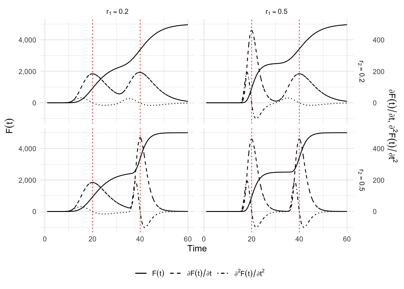

Figure 6.6: Illustration of a Double Gompertz model for different values for $r_{1}$ and $r_{2}$ , with $K_{1} = 2, 500$ , $K_{2} = 5, 000$ , $τ_{1} = 20$ , and $τ_{2} = 40$

6.2.3 Double Richards Model

The double Richards function, its first and second derivatives with respect to time can be coded as follows:

#' Double Richards
#' 
double_richards_f <- function(theta, x) {
  K1 <- theta[["K1"]]
  tau1 <- theta[["tau1"]]
  r1 <- theta[["r1"]]
  delta1 <- theta[["delta1"]]
  K2 <- theta[["K2"]]
  tau2 <- theta[["tau2"]]
  r2 <- theta[["r2"]]
  delta2 <- theta[["delta2"]]
  
  K1 * (1 + delta1 * exp(-r1 * (x - tau1)))^(-1 / delta1) +
    (K2 - K1) * (1 + delta2 * exp(-r2 * (x - tau2)))^(-1 / delta2)
}

#' Double Richards in two parts
#' 
double_richards_f_2 <- function(theta, x) {
  
  K1 <- theta[["K1"]]
  tau1 <- theta[["tau1"]]
  r1 <- theta[["r1"]]
  delta1 <- theta[["delta1"]]
  K2 <- theta[["K2"]]
  tau2 <- theta[["tau2"]]
  r2 <- theta[["r2"]]
  delta2 <- theta[["delta2"]]
  
  f_1 <- K1 * (1 + delta1 * exp(-r1 * (x - tau1)))^(-1 / delta1)
  f_2 <- (K2 - K1) * (1 + delta2 * exp(-r2 * (x - tau2)))^(-1 / delta2)
  
  tibble(x = x, f_1 = f_1, f_2 = f_2)
}

#' First derivative
#' 
double_richards_f_first_d <- function(theta, x) {
  K1 <- theta[["K1"]]
  tau1 <- theta[["tau1"]]
  r1 <- theta[["r1"]]
  delta1 <- theta[["delta1"]]
  K2 <- theta[["K2"]]
  tau2 <- theta[["tau2"]]
  r2 <- theta[["r2"]]
  delta2 <- theta[["delta2"]]
  
  r1 * K1 * exp(-r1 * (x - tau1)) * 
    (delta1 * exp(-r1 * (x - tau1)) + 1)^(-1/delta1 - 1) +
    r2 * (K2-K1) * exp(-r2 * (x - tau2)) * 
    (delta2 * exp(-r2 * (x - tau2)) + 1)^(-1/delta2 - 1)
}

#' Second derivative
#' 
double_richards_f_second_d <- function(theta, x) {
  K1 <- theta[["K1"]]
  tau1 <- theta[["tau1"]]
  r1 <- theta[["r1"]]
  delta1 <- theta[["delta1"]]
  K2 <- theta[["K2"]]
  tau2 <- theta[["tau2"]]
  r2 <- theta[["r2"]]
  delta2 <- theta[["delta2"]]
  
  K1 * (r1^2 * (-1/delta1 - 1) * delta1 * (-exp(-2 * r1 * (x - tau1))) * 
          (delta1 * exp(-r1 * (x - tau1)) + 1)^(-1/delta1 - 2) - r1^2 * 
          exp(-r1 * (x - tau1)) * 
          (delta1 * exp(-r1 * (x - tau1)) + 1)^(-1/delta1 - 1)) +
    
    (K2 - K1) * 
    (r2^2 * (-1 / delta2 - 1) * 
       delta2 * (-exp(-2 * r2 * (x - tau2))) * 
       (delta2 * exp(-r2 * (x - tau2)) + 1)^(-1/delta2 - 2) - 
       r2^2 * 
       exp(-r2 * (x - tau2)) * 
       (delta2 * exp(-r2 * (x - tau2)) + 1)^(-1/delta2 - 1))
}

Let us make some illustrations by varying $r_{1}$ and $r_{2}$ .

situations <- 
  expand_grid(r1 = c(.2, .5), r2 = c(.2, .5)) |> 
  mutate(
    K1     = 2500,
    K2     = 5000,
    tau1   = 20,
    tau2   = 40,
    delta1 = .5,
    delta2 = .5
  )

The function that simulates $C (t)$ and its first and second derivatives with respect to time for a single scenario:

#' Simulation of the logistic model for some parameters
#' 
#' @param i row number of situations
simu <- function(i) {
  current_params <- situations |> slice(i)
  current_params <- c(as_vector(current_params)) |> as.list()
  
  n <- 60
  step <- .01
  sim <-  double_richards_f(
    theta = current_params, x = seq(1,n, by = step))
  simD <-  double_richards_f_first_d(
    theta = current_params, x = seq(1,n, by = step))
  simD2 <-  double_richards_f_second_d(
    theta = current_params, x = seq(1,n, by = step))
  
  tibble(
    t = seq(1, n, by = step),
    K1 = current_params[["K1"]],
    r1 = current_params[["r1"]],
    tau1 = current_params[["tau1"]],
    delta1 = current_params[["delta1"]],
    K2 = current_params[["K2"]],
    r2 = current_params["r2"],
    tau2 = current_params[["tau2"]],
    delta2 = current_params[["delta2"]],
    sim = sim) |> 
    mutate(simD = simD,
           simD2 = simD2)
  
}

Let us apply this function to all scenarios:

simu_res <- map_df(1:nrow(situations), simu)

The thresholds:

threshold_times <- 
  simu_res |> 
  group_by(K1, tau1, r1, K2, tau2, r2, delta1, delta2) |> 
  summarise(threshold_time_1 = unique(tau1),
            threshold_time_2 = unique(tau2)) |> 
  ungroup() |> 
  mutate(
    r1 = str_c("$\\r_1 = ", r1, "$"),
    r2 = str_c("$\\r_2 = ", r2, "$")
  )

`summarise()` has grouped output by 'K1', 'tau1', 'r1', 'K2', 'tau2', 'r2',
'delta1'. You can override using the `.groups` argument.

And the the plots:

p_simu_double_richards <- 
  ggplot(
    data =  simu_res |> 
      mutate(r1 = str_c("$\\r_1 = ", r1, "$"),
             r2 = str_c("$\\r_2 = ", r2, "$")
      ),
    mapping = aes(x = t)) +
  geom_line(aes(y = sim, linetype = "sim")) +
  geom_line(aes(y = simD*10, linetype = "simD")) +
  geom_line(aes(y = simD2*10, linetype = "simD2")) +
  geom_vline(
    data = threshold_times, 
    mapping = aes(xintercept = threshold_time_1),
    colour = "red", linetype = "dotted") +
  geom_vline(
    data = threshold_times,
    mapping = aes(xintercept = threshold_time_2),
    colour = "red", linetype = "dotted") +
  facet_grid(
    r2 ~ r1,
    labeller = as_labeller(
      latex2exp::TeX, 
      default = label_parsed
    )
  ) +
  labs(x = "Time", y = latex2exp::TeX("$F(t)$")) +
  scale_y_continuous(
    labels = comma,
    sec.axis = sec_axis(
      ~./10, 
      name = latex2exp::TeX(
        "$\\partial F(t) / \\partial t$, $\\partial^2 F(t) / \\partial t^2$"
      ),
      labels = comma)) +
  scale_linetype_manual(
    NULL,
    values = c("sim" = "solid", "simD" = "dashed", "simD2" = "dotdash"),
    labels = c("sim" = latex2exp::TeX("$F(t)$"),
               "simD" = latex2exp::TeX("$\\partial F(t) / \\partial t$"),
               "simD2" = latex2exp::TeX("$\\partial^2 F(t) / \\partial t^2$"))
    ) +
  theme(axis.ticks.y = element_blank())

p_simu_double_richards +
  theme_minimal() +
  theme(legend.position = "bottom")

Figure 6.7: Illustration of a Double Richards model for different values for $r_{1}$ and $r_{2}$ , with $K_{1} = 2, 500$ , $K_{2} = 5, 000$ , $τ_{1} = 20$ , $τ_{2} = 40$ “, $δ_{1} = δ_{2} = .5$

Bock, R. Darrell, Howard Wainer, Anne Petersen, David Thissen, James Murray, and Alex Roche. 1973. “A Parameterization for Individual Human Growth Curves.” Human Biology 45 (1): 63–80. http://www.jstor.org/stable/41459847.

Gompertz, Benjamin. 1825. “On the Nature of the Function Expressive of the Law of Human Mortality, and on a New Mode of Determining the Value of Life Contingencies.” Philosophical Transactions of the Royal Society of London 115 (December): 513–83. https://doi.org/10.1098/rstl.1825.0026.

Lee, Se Yoon, Bowen Lei, and Bani Mallick. 2020. “Estimation of COVID-19 Spread Curves Integrating Global Data and Borrowing Information.” PLOS ONE 15 (7): e0236860. https://doi.org/10.1371/journal.pone.0236860.

Lipovetsky, Stan. 2010. “Double Logistic Curve in Regression Modeling.” Journal of Applied Statistics 37 (11): 1785–93. https://doi.org/10.1080/02664760903093633.

Ma, Junling. 2020. “Estimating Epidemic Exponential Growth Rate and Basic Reproduction Number.” Infectious Disease Modelling 5 (January): 129–41. https://doi.org/10.1016/j.idm.2019.12.009.

Oswald, Stephen A., Ian C. T. Nisbet, Andre Chiaradia, and Jennifer M. Arnold. 2012. “FlexParamCurve: R Package for Flexible Fitting of Nonlinear Parametric Curves.” Methods in Ecology and Evolution 3 (6): 1073–77. https://doi.org/10.1111/j.2041-210x.2012.00231.x.

Richards, F. J. 1959. “A Flexible Growth Function for Empirical Use.” Journal of Experimental Botany 10 (2): 290–301. https://doi.org/10.1093/jxb/10.2.290.

Thissen, David, R. Darrell Bock, Howard Wainer, and Alex F. Roche. 1976. “Individual Growth in Stature: A Comparison of Four Growth Studies in the U.S.A.” Annals of Human Biology 3 (6): 529–42. https://doi.org/10.1080/03014467600001791.

Tjørve, Kathleen M. C., and Even Tjørve. 2017. “The Use of Gompertz Models in Growth Analyses, and New Gompertz-Model Approach: An Addition to the Unified-Richards Family.” PLOS ONE 12 (6): e0178691. https://doi.org/10.1371/journal.pone.0178691.

Tsoularis, A., and J. Wallace. 2002. “Analysis of Logistic Growth Models.” Mathematical Biosciences 179 (1): 21–55. https://doi.org/10.1016/S0025-5564(02)00096-2.

Verhulst, P. F. 1845. “Recherches Mathématiques Sur La Loi d’accroissement de La Population.” Nouveaux mémoires de l’Académie Royale Des Sciences Et Belles-Lettres de Bruxelles 18: 14–54. https://eudml.org/doc/182533.

Wang, Xiang-Sheng, Jianhong Wu, and Yong Yang. 2012. “Richards Model Revisited: Validation by and Application to Infection Dynamics.” Journal of Theoretical Biology 313: 12–19. https://doi.org/10.1016/j.jtbi.2012.07.024.