In this chapter, we use R to make an animated version of the simulation of the epidemics using the SIR model.
── Attaching core tidyverse packages ──────────────────────── tidyverse 2.0.0 ──
✔ dplyr     1.1.2     ✔ readr     2.1.4
✔ forcats   1.0.0     ✔ stringr   1.5.0
✔ ggplot2   3.4.2     ✔ tibble    3.2.1
✔ lubridate 1.9.2     ✔ tidyr     1.3.0
✔ purrr     1.0.1
── Conflicts ────────────────────────────────────────── tidyverse_conflicts() ──
✖ dplyr::filter() masks stats::filter()
✖ dplyr::lag()    masks stats::lag()
ℹ Use the conflicted package (<http://conflicted.r-lib.org/>) to force all conflicts to become errors
Loading required package: sp

Attaching package: 'raster'

The following object is masked from 'package:dplyr':

    select
We will consider that individuals live on a square with sides of 5.
Each time unit, individuals can take a step. The size of the step is defined with the following variable:
<- abs (max (bounds)- min (bounds))/ 30
Let us set some key parameters of the epidemics:
The probability that a \(S\) gets infected while in contact with an \(I\) is set here to .8
To be infected, we consider a radius of .5 around an \(I\) .
At the beginning of the simulation, the number of infected is set to .02.
Once an individual has been infected, it takes 7 periods before it turns to \(R\) .
<- 0.8 <- 0.5 <- 0.02 <- 7
Let us consider \(N=150\) individuals, and a time span of 100 periods.
The position of the individuals will be stored in the following object:
<- vector (mode = "list" , length = nsteps)
The initial positions are randomly drawn from a Uniform distribution \(\mathcal{U}(-5,5)\) .
set.seed (123 )<- runif (n = n, min = min (bounds), max = max (bounds))<- runif (n = n, min = min (bounds), max = max (bounds))
At each moment, let us store the status of the infected in an object called status. Here are the random status at the beginning. On average, if we replicate the analysis multiple times, the proportion of infected at the beginning of the epidemic should be equal to \(0.02\) .
<- sample (c ("S" , "I" ),replace = TRUE , size = round (n), prob = c (1 - I_0, I_0)table (status)prop.table (table (status))
The number of infected at the beginning:
<- sum (status == "I" )
Let us store the current state of our simulated world in a tibble:
<- tibble (x = x, y = y, step = 1 , status = status)
At each time, the state of the world will be stored in the ith element of positions.
1 ]] <- df_current
We need to identify the individuals with respect to their status:
<- which (df_current$ status == "I" )<- which (df_current$ status == "S" )<- NULL
The time since infection is set to 0 for all individuals…
<- rep (0 , n)
… except for those that are infected at the first period.For those, the time to infection is set to 1:
<- 1
Then we can begin the loop over the periods.
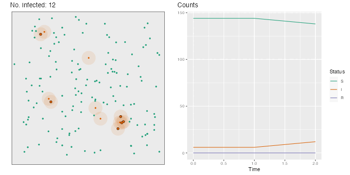
for (i in 2 : nsteps) {# Movements, in both directions <- runif (n = n, min = - step_size, max = step_size)<- runif (n = n, min = - step_size, max = step_size)<- x+ deplacement_x<- y+ deplacement_y> max (x)] <- max (bounds)< min (x)] <- min (bounds)> max (y)] <- max (bounds)< min (y)] <- min (bounds)# Recovery <- which (time_since_infection> time_recovery)if (length (id_new_recovered) > 0 ) {<- c (id_R, id_new_recovered)<- id_I[! id_I %in% id_new_recovered]<- "R" <- 0 # New infections <- pointDistance (cbind (x[id_I], y[id_I]),cbind (x[id_S], y[id_S]),lonlat= FALSE # Identifying close individuals <- which (dist_matrix < radius_infec, arr.ind = TRUE )if (length (close_points) > 0 ) {<- id_S[close_points[,"col" ]]<- sample (c (TRUE , FALSE ), size = nrow (close_points), prob = c (proba_infect, 1 - proba_infect), replace = TRUE <- ids_potential_new_infected[are_infected]!= 0 ] <- != 0 ] + 1 <- 1 <- sort (c (id_I, ids_new_infected))<- "I" <- id_S[! id_S %in% ids_new_infected]# Storing the current state of the world <- tibble (x = x, y = y, step = i, status = status) |> mutate (status = factor (status, levels = c ("S" , "I" , "R" )))# Plotting the situation <- ggplot (data = positions[[i]], mapping = (aes (x = x, y = y, colour = status))) + :: geom_circle (data = positions[[i]] |> filter (status == "I" ) |> mutate (r = radius_infec),mapping = aes (x0 = x, y0 = y, r = rfill = "#d95f02" ,colour = NA ,alpha = .1 ,inherit.aes = FALSE + geom_point (size = 1 ) + labs (x = "" , y = NULL , title = str_c ("No. Infected: " , length (id_I))) + coord_equal (xlim = bounds, ylim = bounds) + scale_colour_manual ("Status" , values = c ("S" = "#1b9e77" ,"I" = "#d95f02" ,"R" = "#7570b3" guide = "none" ) + theme (plot.title.position = "plot" , panel.border = element_rect (linetype = "solid" , fill= NA ),panel.grid = element_blank (),axis.ticks = element_blank (),axis.text = element_blank ()if (length (close_points) > 0 ) {if (length (ids_new_infected) > 0 ) {<- p + geom_point (data = positions[[i]] |> slice (ids_new_infected),mapping = aes (x = x, y = y),size = 2 , colour = "black" + geom_point (data = positions[[i]] |> slice (ids_new_infected),mapping = aes (x = x, y = y),size = 1.5 <- map_df (1 : i],~ group_by (., status) |> count (),.id = "time" |> ungroup () |> bind_rows (tibble (time = "0" ,status = c ("S" , "I" , "R" ), n = c (n - nb_infected_start, nb_infected_start, 0 )|> complete (status, time) |> mutate (n = replace_na (n, 0 ),time = as.numeric (time),status = factor (status, levels = c ("S" , "I" , "R" ))<- ggplot (data = df_plot,mapping = aes (x = time, y = n, colour = status)) + geom_line () + scale_colour_manual ("Status" , values = c ("S" = "#1b9e77" ,"I" = "#d95f02" ,"R" = "#7570b3" + labs (x = "Time" , y = NULL , title = "Counts" ) + theme (plot.title.position = "plot" )<- cowplot:: plot_grid (p, p_counts)<- str_c ("figs/simul_" ,str_pad (i, width = 3 , side = "left" , pad = 0 ),".png" :: save_plot (filename = file_name,ncol = 2 ,base_asp = 1.1 ,base_width = 5 ,base_height = 5 ,dpi= 72
The png files can be merged in a gif file with a system command:
system ("convert figs/*.png figs/animation-sir.gif" )
The resulting gif can be seen in Figure 3.1 .
if (knitr:: is_html_output ()) {:: include_graphics ("figs/animation-sir.gif" )else if (knitr:: is_latex_output ()) {:: include_graphics ("figs/simul_100.png" )