16  Descriptive Statistics

Objectives

This chapter presents descriptive statistics on the data. It shows the distribution of the MHI-5 and MHI-3 scores in the sample. Some statistics about all the variables are given on the whole sample and on sub-samples defined according to the classification of people given their MHI-5 score. We use self-assessed health status instead of depression here.

Let us load:

Let us first load {tidyverse}:

library(tidyverse)
── Attaching core tidyverse packages ──────────────────────── tidyverse 2.0.0 ──
✔ dplyr     1.1.4     ✔ readr     2.1.5
✔ forcats   1.0.0     ✔ stringr   1.5.1
✔ ggplot2   3.5.1     ✔ tibble    3.2.1
✔ lubridate 1.9.3     ✔ tidyr     1.3.1
✔ purrr     1.0.2     
── Conflicts ────────────────────────────────────────── tidyverse_conflicts() ──
✖ dplyr::filter() masks stats::filter()
✖ dplyr::lag()    masks stats::lag()
ℹ Use the conflicted package (<http://conflicted.r-lib.org/>) to force all conflicts to become errors

The raw data:

load("../data/df_merged.rda")
dim(df)
[1] 18561   841

Then the cleaned data:

load("../data/df_clean_sah.rda")
dim(df_clean)
[1] 5380   94

Let us add a variable in df stating whether or not the observation is included in the final sample:

df <- df |> 
  mutate(in_sample = id %in% df_clean$id)

Sanity check:

table(df$in_sample)

FALSE  TRUE 
13181  5380 

Let us get the name of each variable, as defined in [Chapter -Chapter 2)

load("../data/out/variable_names.rda")

Let us change the Not reported and Not surveyed variables to No answer:

df <- 
  df |> 
  mutate(
    across(
      .cols = is.factor,
      .fns = function(x) {
        fct_recode(x,
                   "No answer" = "Not reported",
                   "No answer" = "Not surveyed"
        )
      }
    )
  )

16.1 MHI-Scores

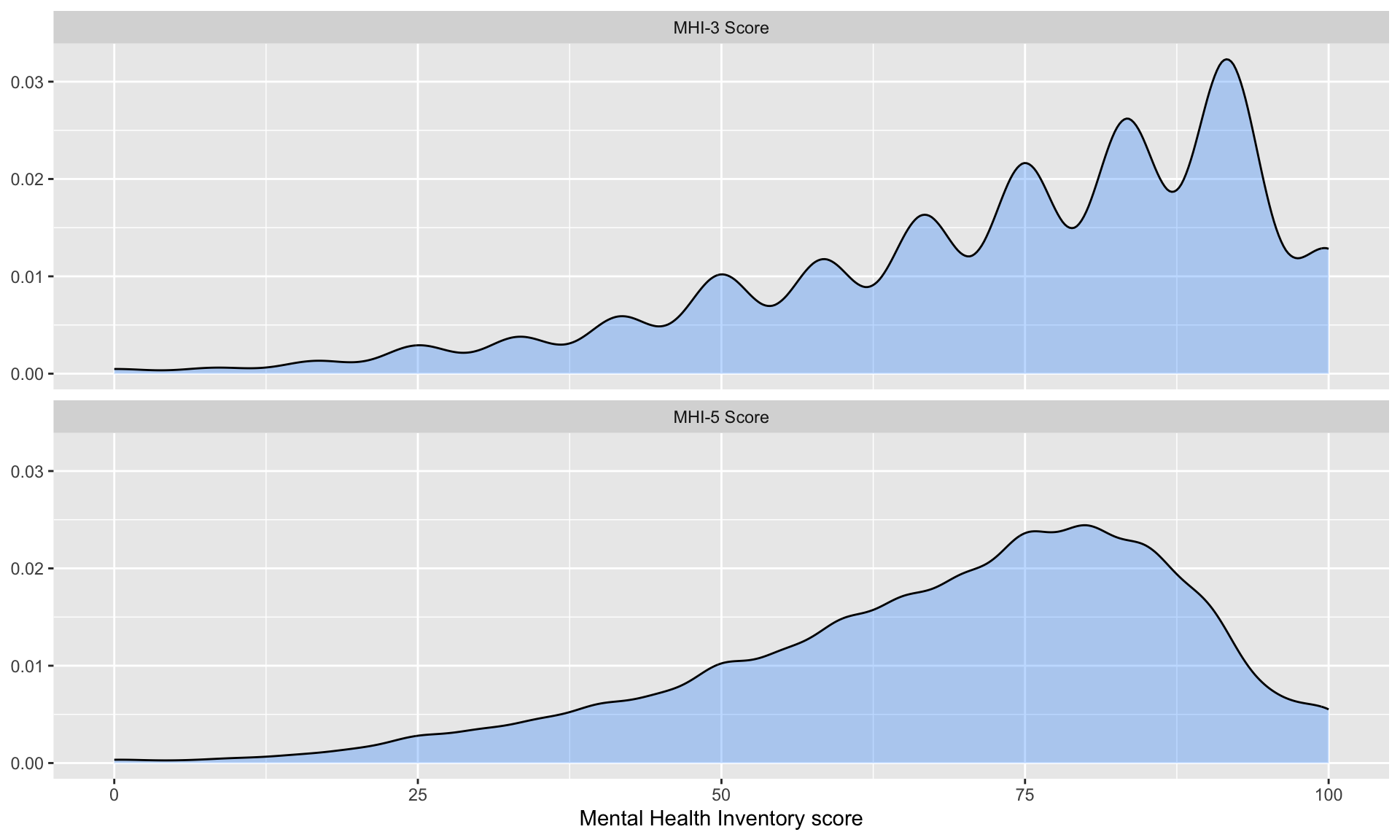
We can first look at the distribution of the MHI-5 and MHI-3 scores over the entire dataset. Due to the construction of the MHI scores, one notes relatively high masses for multiples of 5. The distribution of MHI scores is skewed on the right both for MHI-3 and MHI-5.

df |> 
  group_by(PERSONNE_etat_sante) |> 
  summarise(
    mhi_5_mean = mean(score_t_corrected, na.rm=T),
    mhi_5_sd = sd(score_t_corrected, na.rm=T),
    n = n()
  )
# A tibble: 3 × 4
  PERSONNE_etat_sante            mhi_5_mean mhi_5_sd     n
  <chr>                               <dbl>    <dbl> <int>
1 Not reported                         61.8     22.1  5430
2 Very Bad or Bad                      46.8     21.4   929
3 Very Good, Good or Fairly Good       70.7     17.4 12202
Show the codes to create the graph
ggplot(
  data = df |> 
  select(PERSONNE_score_t_corrected, score_mhi_3) |> 
  rename(
    "MHI-5 Score" = PERSONNE_score_t_corrected,
    "MHI-3 Score" = score_mhi_3
  ) |> 
  gather(score, value, `MHI-5 Score`, `MHI-3 Score`), 
  mapping = aes(x = value)
  ) +
  geom_density(alpha = .3, fill = "dodger blue") +
  labs(
    x = "Mental Health Inventory score", y = NULL
  ) +
  facet_wrap(~score, ncol = 1) +
  theme(
    plot.title.position = "plot",
    plot.title = element_text(hjust = 0, size = rel(1.3), face = "bold")
  )
Warning: Removed 12376 rows containing non-finite outside the scale range
(`stat_density()`).
Figure 16.1: Density of MHI-5 and MHI-3 scores
Show the codes to create the graph
ggplot(data = df |> 
  filter(in_sample) |> 
  select(PERSONNE_score_t_corrected, score_mhi_3) |> 
  rename("MHI-5 Score" = PERSONNE_score_t_corrected, "MHI-3 Score" = score_mhi_3) |> 
  gather(score, value, `MHI-5 Score`, `MHI-3 Score`), 
  mapping = aes(x = value)
) +
  geom_density(alpha = .3, fill = "dodger blue") +
  labs(
    x = "Mental Health Inventory score", y = NULL) +
  facet_wrap(~score, ncol = 1)
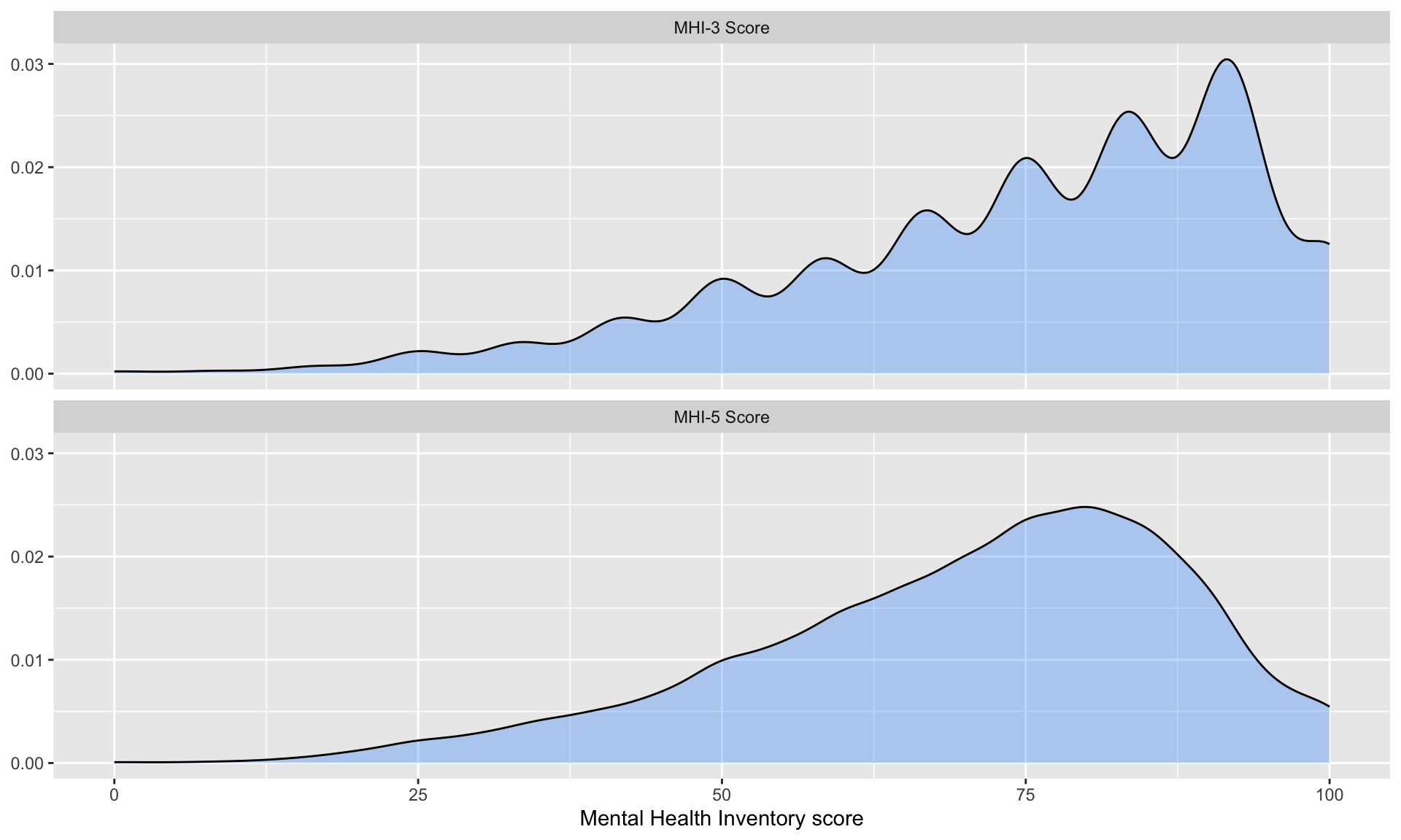
Figure 16.2: Density of MHI-5 and MHI-3 scores

Respondents to the ESPS survey answered the following question: “In the past 12 months, have you experienced depression?” (“Au cours des 12 derniers mois, avez-vous eu une dépression?”).

The responses are distributed as follows:

# Counts
table(df$PERSONNE_etat_sante)

                  Not reported                Very Bad or Bad 
                          5430                            929 
Very Good, Good or Fairly Good 
                         12202 
# Proportions
prop.table(table(df$PERSONNE_etat_sante)) |> round(2)

                  Not reported                Very Bad or Bad 
                          0.29                           0.05 
Very Good, Good or Fairly Good 
                          0.66 
Note

Recall that in the sample used, we focus on individuals who reported a good health status.

# Counts
df |> 
  filter(in_sample) |>
  pull(PERSONNE_etat_sante) |> 
  table()

Very Good, Good or Fairly Good 
                          5380 
# Proportions
df |> 
  filter(in_sample) |>
  pull(PERSONNE_etat_sante) |> 
  table() |> 
  prop.table() |> 
  round(digits = 2)

Very Good, Good or Fairly Good 
                             1 

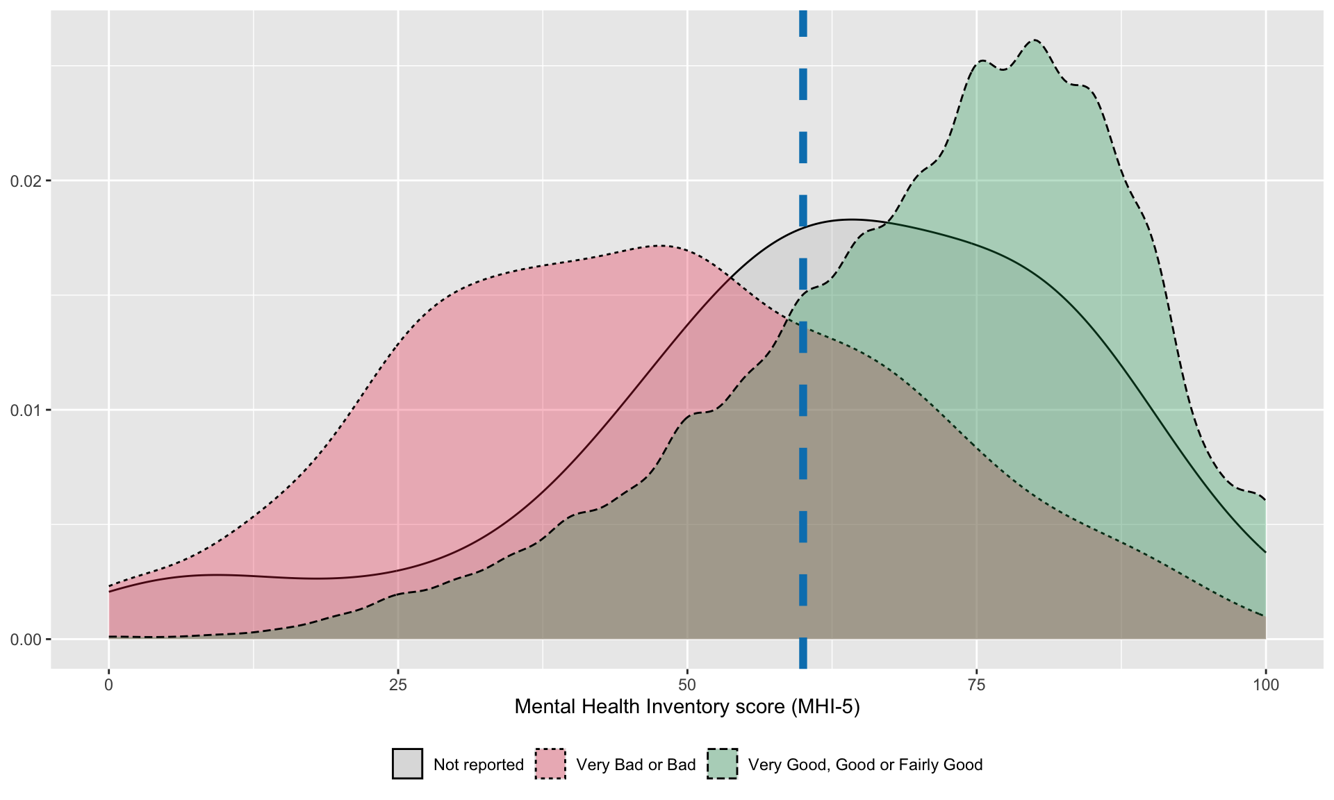
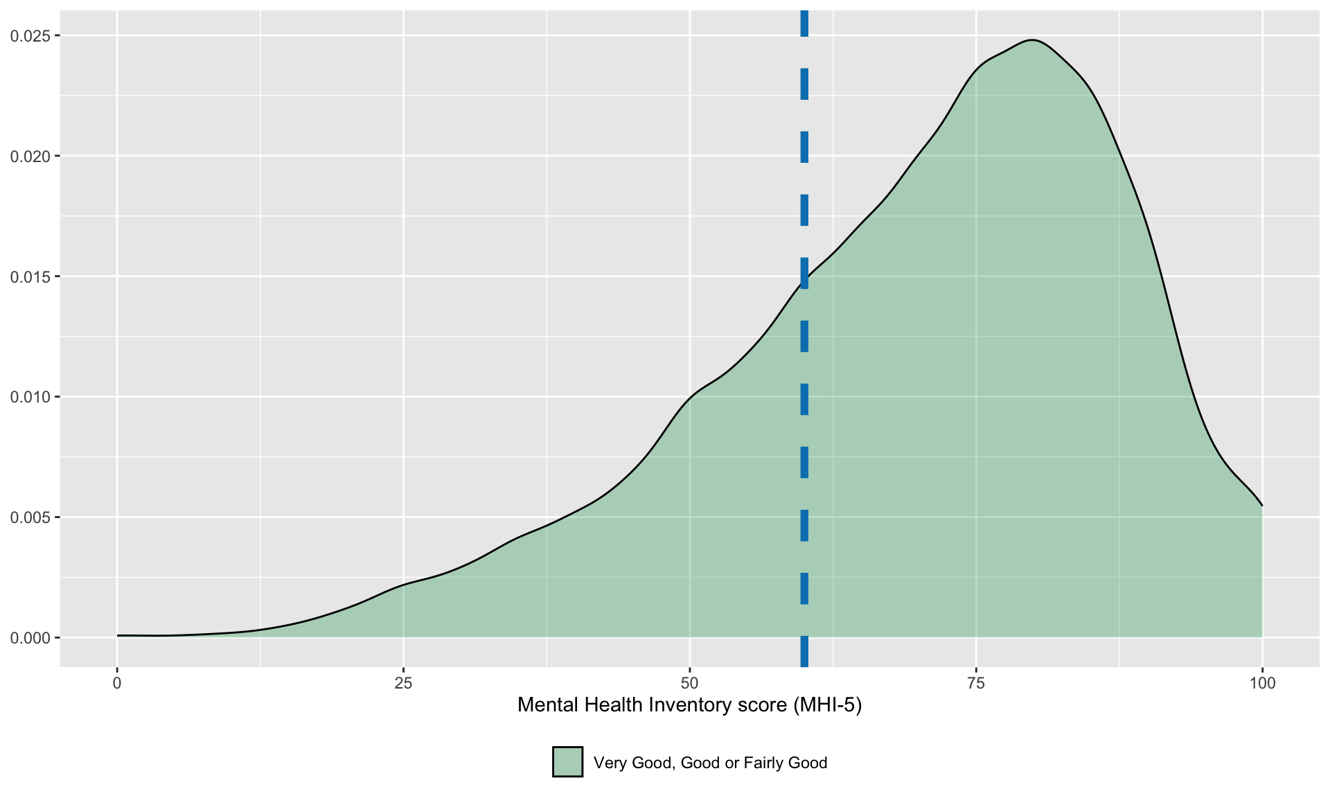
Let us examine the distribution of the MHI-5 score by grouping individuals according to their response to the question regarding depression. Let us add a vertical dashed line on the graph corresponding to the first quartile of the overall distribution of MHI-5 scores.

Show the codes to create the graph
p_distrib_mhi_5 <- ggplot(
    data = df,
    mapping = aes(x = PERSONNE_score_t_corrected)
  ) +
  geom_density(
    mapping = aes(fill = PERSONNE_etat_sante, linetype = PERSONNE_etat_sante), 
    alpha = .3
  ) +
  geom_vline(
    xintercept = quantile(
      df$PERSONNE_score_t_corrected,
      probs = .25, 
      na.rm = TRUE
    ),
    colour = "#0081BC", linetype = "dashed", linewidth = 2
  ) +
  labs(x = "Mental Health Inventory score (MHI-5)", y = NULL) +
  scale_fill_manual(
    NULL,
    values = c(
      "Very Good, Good or Fairly Good" = "#009D57",
      "Very Bad or Bad" = "#EE324E",
      "Not reported" = "grey"
    )
  ) +
  scale_linetype_discrete(NULL) +
  theme(legend.position = "bottom")

p_distrib_mhi_5
Warning: Removed 6188 rows containing non-finite outside the scale range
(`stat_density()`).
Figure 16.3: Density of MHI-5 scores
Show the codes to create the graph
p_distrib_mhi_5 <- 
  ggplot(
    data = df |> 
  filter(in_sample),
  mapping = aes(x = PERSONNE_score_t_corrected)
  ) +
  geom_density(
    mapping = aes(fill = PERSONNE_etat_sante, linetype = PERSONNE_etat_sante), 
    alpha = .3
  ) +
  geom_vline(
    xintercept = quantile(
      df$PERSONNE_score_t_corrected, probs = .25, 
      na.rm = TRUE
    ),
    colour = "#0081BC", linetype = "dashed", size = 2
  ) +
  labs(x = "Mental Health Inventory score (MHI-5)", y = NULL) +
  scale_fill_manual(
    NULL, 
    values = c(
      "Very Good, Good or Fairly Good" = "#009D57",
      "Very Bad or Bad" = "#EE324E",
      "Not reported" = "grey"
    )
  ) +
  scale_linetype_discrete(NULL) +
  theme(legend.position = "bottom")
Warning: Using `size` aesthetic for lines was deprecated in ggplot2 3.4.0.
ℹ Please use `linewidth` instead.
Show the codes to create the graph
p_distrib_mhi_5
Figure 16.4: Density of MHI-5 scores

Recall that we used the first quartile as the threshold for the classification of individuals as either “low” MHI score or “high” MHI score. The first quantile is:

quant <- .25
q1_mhi_5 <- quantile(df$PERSONNE_score_t_corrected, probs = quant, na.rm=TRUE)
q1_mhi_5
25% 
 60 

We decided to remove from the dataset the individuals who did not answer the question regarding their health status, leaving us with the following distribution:

tableau_size <- 
  df |> 
  filter(PERSONNE_age >= 15) |> 
  filter(!is.na(PERSONNE_score_t_corrected)) |> 
  filter(PERSONNE_etat_sante != "Not reported") |> 
  mutate(
    PERSONNE_etat_sante = factor(
      PERSONNE_etat_sante, 
      levels = c("Very Bad or Bad", "Very Good, Good or Fairly Good")
    )
  ) |> 
  mutate(inf_q1 = PERSONNE_score_t_corrected <= q1_mhi_5) |> 
  mutate(
    inf_q1 = factor(inf_q1, levels = c(T,F), 
                    labels = c("MHI-5 <= Q1", "MHI-5 > Q1")
    )
  ) |> 
  ungroup()

tableau_size_2 <- table(tableau_size$inf_q1, tableau_size$PERSONNE_etat_sante)
(tableau_size_2_margins <- addmargins(tableau_size_2))
             
              Very Bad or Bad Very Good, Good or Fairly Good   Sum
  MHI-5 <= Q1             633                           3246  3879
  MHI-5 > Q1              212                           8213  8425
  Sum                     845                          11459 12304
round(prop.table(tableau_size_2)*100,1)
             
              Very Bad or Bad Very Good, Good or Fairly Good
  MHI-5 <= Q1             5.1                           26.4
  MHI-5 > Q1              1.7                           66.8
tableau_size_sample <- 
  df |> 
  filter(in_sample) |> 
  filter(!is.na(PERSONNE_score_t_corrected)) |> 
  filter(PERSONNE_etat_sante != "Not reported") |> 
  mutate(
    PERSONNE_etat_sante = factor(
      PERSONNE_etat_sante, 
      levels = c("Very Bad or Bad", "Very Good, Good or Fairly Good")
    )
  ) |> 
  mutate(inf_q1 = PERSONNE_score_t_corrected <= q1_mhi_5) |> 
  mutate(
    inf_q1 = factor(
      inf_q1, levels = c(T,F), 
      labels = c("MHI-5 <= Q1", "MHI-5 > Q1")
    )
  )|> 
  ungroup()

tableau_size_sample_2 <- table(tableau_size_sample$inf_q1, tableau_size_sample$PERSONNE_pb_depress)
(tableau_size_sample_2_margins <- addmargins(tableau_size_sample_2))
             
              No depression Depression No answer  Sum
  MHI-5 <= Q1          1336        198        58 1592
  MHI-5 > Q1           3591         50       147 3788
  Sum                  4927        248       205 5380
round(prop.table(tableau_size_sample_2)*100,1)
             
              No depression Depression No answer
  MHI-5 <= Q1          24.8        3.7       1.1
  MHI-5 > Q1           66.7        0.9       2.7

In the study, we decided to use the first quartile of the distribution of MHI-5 scores to classify individuals as depressed (when their MHI-5 score is less than or equal to the first quartile of the distribution) or non-depressed (when their MHI-5 score is greater than the first quartile of the distribution). In this robustness test, we replaced the question about depression by the self-assessed health status. It is possible to illustrates the impact of the choice of the cut-off used on the MHI-5 score on the proportion of individuals designated as in bad health or not with respect to the MHI-5 score. To that end, we can first create a function that computes the proportion of people classified as depending on the selected threshold.

get_prop <- function(prob, df) {
  q1_mhi_5 <- quantile(df$PERSONNE_score_t_corrected, probs = prob, na.rm=TRUE)
  tableau <- df |> 
    filter(!is.na(PERSONNE_score_t_corrected)) |> 
    filter(PERSONNE_etat_sante != "Not reported") |> 
    mutate(inf_q1 = PERSONNE_score_t_corrected <= q1_mhi_5) |> 
    group_by(PERSONNE_etat_sante) |> 
    summarise(inf_q1 = sum(inf_q1),
              sup_q1 = n() - inf_q1,
              tot = n()) |> 
    mutate(inf_q1_prop = inf_q1 / (inf_q1 + sup_q1),
           inf_q1_prop = round(inf_q1_prop*100, 2))
  
  nb_inf_q1 <- tableau |> 
    filter(PERSONNE_etat_sante == "Very Good, Good or Fairly Good") |> 
    pull(inf_q1)
  
  nb_sup_q1 <- tableau |> 
    filter(PERSONNE_etat_sante == "Very Good, Good or Fairly Good") |> 
    pull(sup_q1)
  
  
  nb_obs_depression <- tableau |> 
    filter(PERSONNE_etat_sante == "Very Good, Good or Fairly Good") |> 
    pull(tot)
  
  tibble(
    prob = prob, 
    cutoff = q1_mhi_5, 
    prop_bad_health_inf = nb_inf_q1 / nb_obs_depression
  )
}

This function can be applied to a sequence of thresholds, ranging from 0 to 1:

prop_badhealth_inf <- 
  map_dfr(.x = seq(0, 1, by = .05), .f = get_prop, df = df)

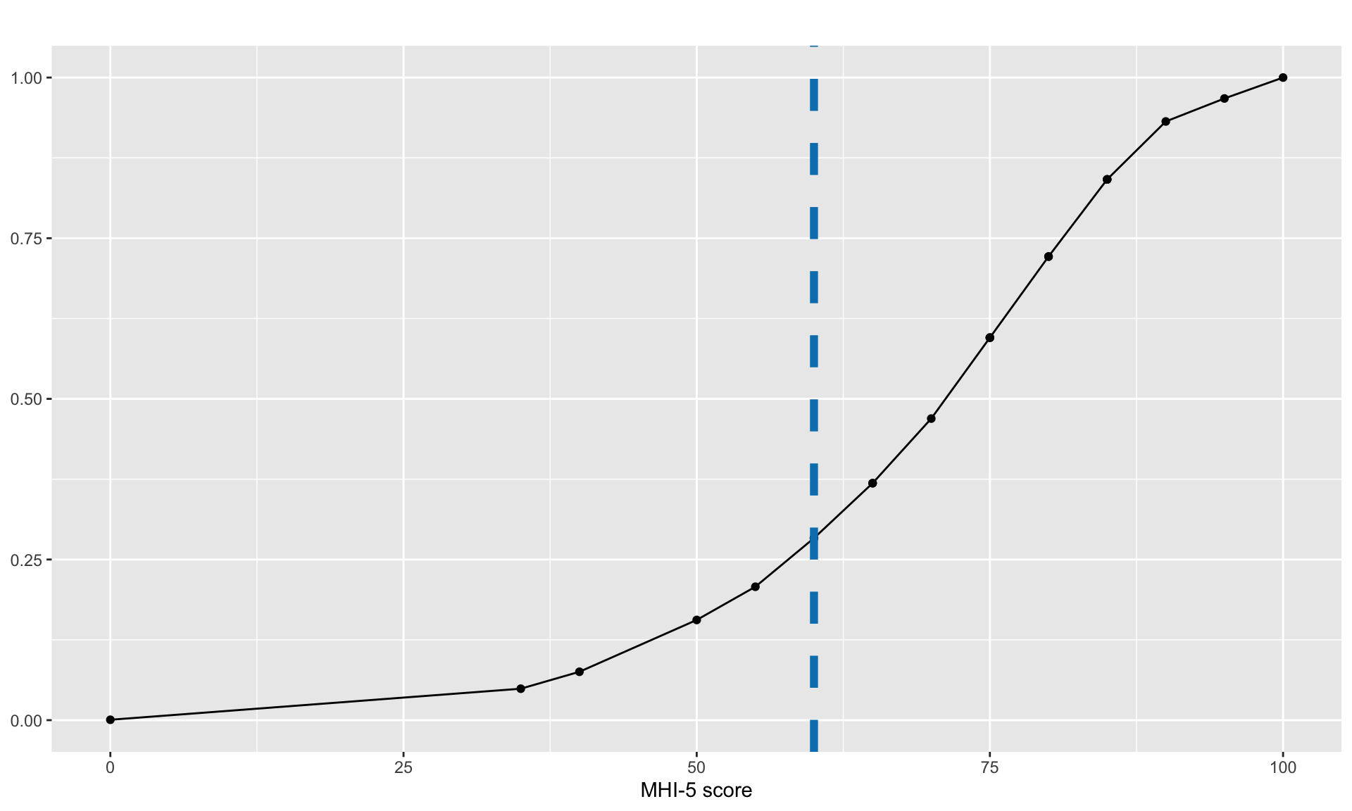
We can plot the proportion of people classified as in bad health as a function of the threshold used on the MHI-5 score. We have added a vertical blue dashed line to show the threshold used, i.e., the first quartile of the MHI-5 score distribution.

Show the codes to create the graph
p_imaginary_healtyh <- 
  ggplot(
    data = prop_badhealth_inf, 
    mapping = aes(x = cutoff, y = prop_bad_health_inf)
  ) +
  geom_line() +
  geom_point() +
  geom_vline(
    xintercept = q1_mhi_5, colour = "#0081BC", linetype = "dashed", size = 2
  ) +
  labs(
    x = "MHI-5 score", y = NULL,
       title = ""
    ) +
  theme(plot.title.position = "plot",
        plot.title = element_text(hjust = 0, size = rel(1.3), face = "bold"))

p_imaginary_healtyh
Figure 16.5: Proportion of individuals classified as i nbad health depending on MHI-5 score
Show the codes to create the graph
p_distrib_ages <- 
  ggplot(
    data = df |> 
  filter(
    PERSONNE_etat_sante %in% c("Very Bad or Bad", "Very Good, Good or Fairly Good"),
    !is.na(inf_q1_mhi_5)
  ) |> 
  mutate(
    PERSONNE_etat_sante = factor(
      PERSONNE_etat_sante,
      levels = c("Very Bad or Bad", "Very Good, Good or Fairly Good")
    )
  ) |> 
  mutate(
    inf_q1_mhi_5 = factor(
      as.character(inf_q1_mhi_5),
      levels = c("<=Q1", ">Q1"),
      labels = c("MHI-5 <= Q1", "MHI-5 >Q1")
    )
  ),
  mapping = aes(x = PERSONNE_age)
  ) +
  geom_density(aes(fill = inf_q1_mhi_5), alpha = .5) +
  labs(x = "Age", y = NULL) +
  scale_fill_manual(
    NULL, values = c(
      "MHI-5 >Q1" = "#009D57",
      "MHI-5 <= Q1" = "#EE324E"
    )
  ) +
  facet_grid(inf_q1_mhi_5 ~ PERSONNE_etat_sante) +
  theme(legend.position = "bottom")
p_distrib_ages
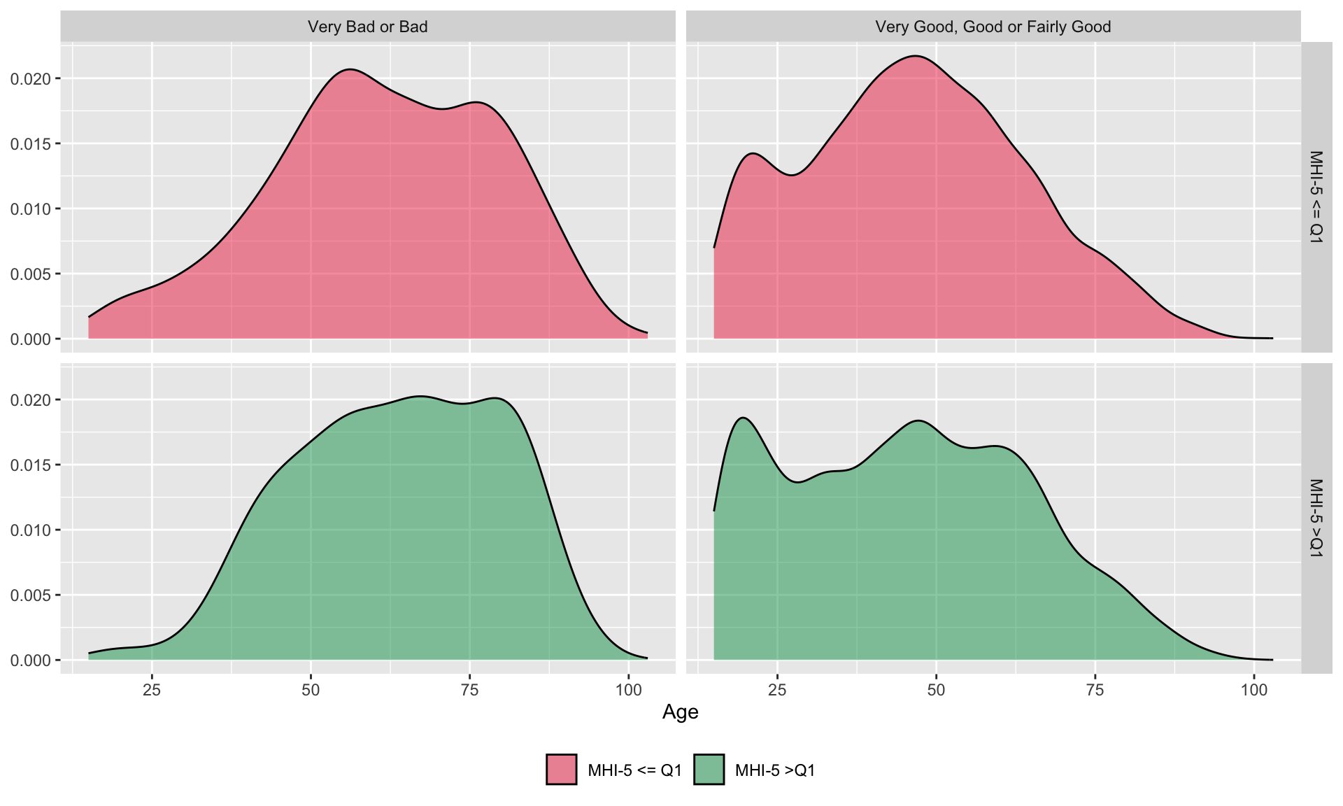
Figure 16.6: Density of age of individuals in each category
Show the codes to create the graph
p_distrib_ages_2 <- 
  ggplot(
    data = df |> 
      filter(in_sample) |> 
      filter(
        PERSONNE_etat_sante %in% c("Very Bad or Bad", "Very Good, Good or Fairly Good"),
        !is.na(inf_q1_mhi_5)
      ) |> 
      mutate(
        PERSONNE_etat_sante = factor(
          PERSONNE_etat_sante,
          levels = c("Very Bad or Bad", "Very Good, Good or Fairly Good")
        )
      ) |> 
      mutate(
        inf_q1_mhi_5 = factor(
          as.character(inf_q1_mhi_5),
          levels = c("<=Q1", ">Q1"),
          labels = c("MHI-5 <= Q1", "MHI-5 >Q1")
        )
      ),
    mapping = aes(x = PERSONNE_age)
  ) +
  geom_density(aes(fill = inf_q1_mhi_5), alpha = .5) +
  labs(x = "Age", y = NULL) +
  scale_fill_manual(
    NULL,
    values = c("MHI-5 >Q1" = "#009D57", "MHI-5 <= Q1" = "#EE324E")
  ) +
  facet_grid(inf_q1_mhi_5 ~ PERSONNE_etat_sante) +
  theme(legend.position = "bottom")

p_distrib_ages_2
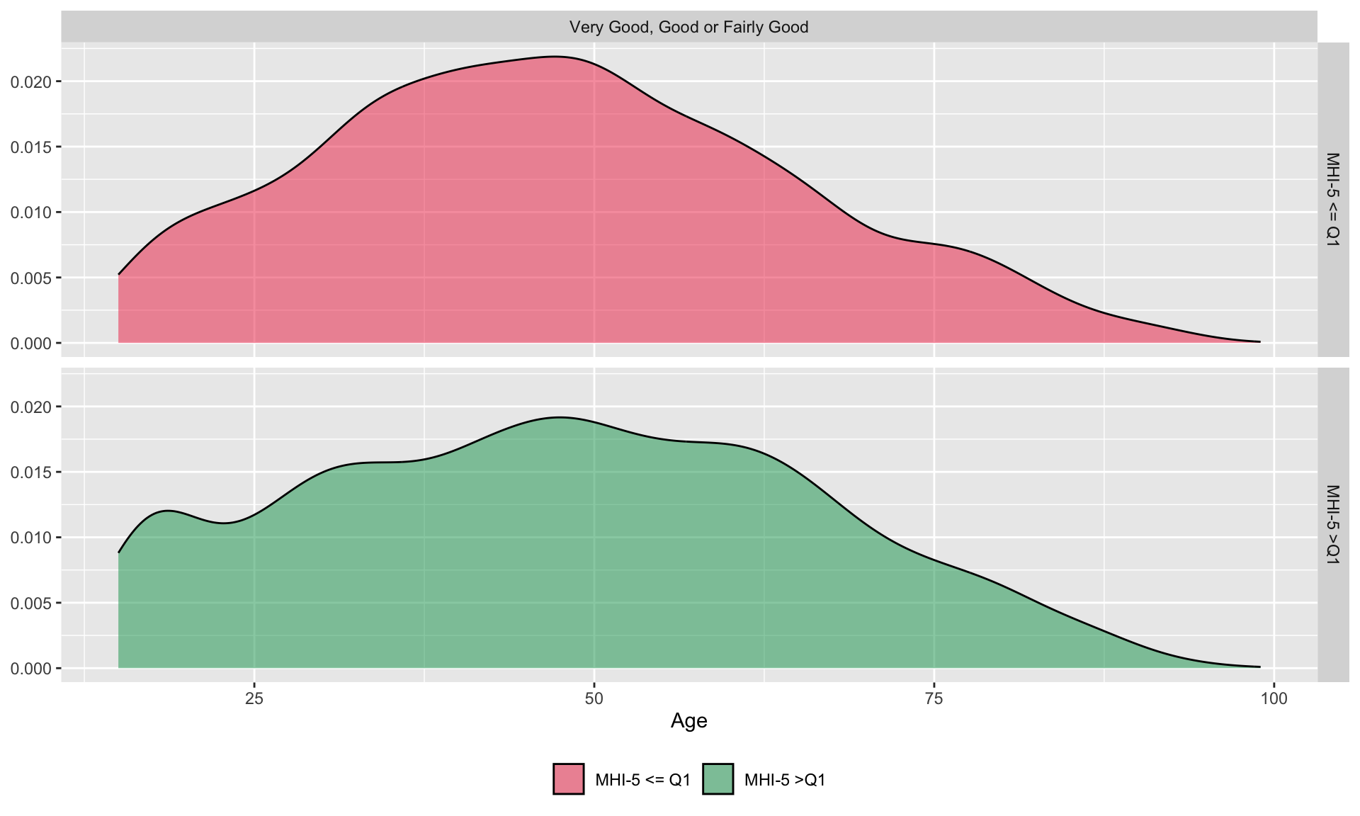
Figure 16.7: Density of age of individuals in each category

16.2 Differences Between Sub-samples

We wish to provide descriptive statistics for sub samples of the data. As the study focuses on people who report a good health status, the descriptive statistics are provided only for these individuals. We consider three different subsets:

  • all the individuals who report they have a Very Good, Good or Fairly Good health

  • among those:

    • individuals with a low MHI-5 score (imaginary healthy)
    • individuals with a high MHI-5.

16.2.1 Heplper Functions

We first create a function that format p-values:

#' format_p_value
#' Format the p-value so that it displays "<10^{i}", if i <= 3
#' rounds the value with 2 digits otherwise
#' @param x p-value to format
#' x <- 0.000133613 ; x <- 0.0011
format_p_value <- function(x) {
  if (x < 10^-3) {
    resul <- str_c("**$< 10^{-3}$**")
  } else if (x > 10^-3) {
    if (x < 0.05) {
      resul <- str_c("**$", round(x, 3), "$**")
    } else {
      resul <- str_c("$", round(x, 3), "$")
    }
  } else {
    resul <- "**$0.001$**"
  }
  
  resul
}

Then, we create a function that provides some summary statistics for that specific variable, depending on its class:

  • if the variable is numerical: the average value
  • if the variable is categorical: the number of observation and the proportion of each category.

These summary statistics are given for each of the three subsets of data described previously. In addition, the results of a test of equality of means (for numerical variables) or proportions (for categorical ones) is provided.

#' sample_diff_depression
#' Compute descriptive statistics on `df` grouped by `grouping_var`
#' depending on the type of the variable of interest (qualitative, ordinal, numerical)
#' Then performs test of equality of mean (or proportion) on the sub-samples.
#' @param variable (string) name of the variable of interest
#' @param grouping_var (string) name of the qualitative variable that defines groups
#' @param type type of the variable (qualitative, ordinal, or numerical)
#' variable <- "PERSONNE_age" ; grouping_var <- "PERSONNE_pb_depress"
sample_diff_sah <- function(variable, 
                                   df, 
                                   grouping_var, 
                                   type = c("qualitative", "ordinal", "numerical")) {
  
  label_variable <- variable_names |> 
    filter(variable == !!variable) |> pull(label)
  
  
  if (type %in% c("qualitative", "ordinal")) {
    
    whole_sample <- 
      df |> 
      filter(!is.na(!!!syms(variable)), !is.na(!!!syms(grouping_var))) |> 
      mutate(label = label_variable) |> 
      select(label, !!!variable) |> 
      group_by(label, !!!syms(variable)) |> 
      summarise(n = n())
    
    nb_tot <- sum(whole_sample$n)
    
    whole_sample <- 
      whole_sample |> 
      mutate(
        pct = n / sum(n),
        pct = (round(100 * pct, 2)),
        pct = str_c("(", pct, "%)")
      ) |> 
      unite(`Whole Sample`, n, pct, sep = " ")
    
    subsamples <- 
      df |> 
      filter(!is.na(!!!syms(variable)), !is.na(!!!syms(grouping_var))) |> 
      mutate(label = label_variable) |> 
      select(label, !!!variable, !!!grouping_var) |> 
      group_by(label, !!!syms(variable), !!!(syms(grouping_var))) |> 
      summarize(n = n()) |> 
      group_by(!!!syms(grouping_var)) |> 
      mutate(
        pct = n / sum(n),
        pct = (round(100 * pct, 2)),
        pct = str_c("(", pct, "%)")
      ) |> 
      unite(value, n, pct, sep = " ")
    
    res <- 
      whole_sample |> 
      left_join(subsamples) |> 
      ungroup() |> 
      spread(
        key = grouping_var, 
        value = "value", 
        fill = "0 (0.00%)"
      ) |> 
      mutate(
        label = ifelse(
          row_number() == 1, 
          yes = str_c(label, " (n = ", format(nb_tot, big.mark = ","), ")"), 
          no = label
        )
      ) |> 
      unite(label, label, !!!variable, sep = " ")
    
  } else {
    
    whole_sample <- 
      df |> 
      filter(!is.na(!!!syms(variable)), !is.na(!!!syms(grouping_var))) |> 
      mutate(label = label_variable) |> 
      select(label, !!!variable)
    
    nb_tot <- nrow(whole_sample)
    
    whole_sample <- 
      whole_sample |> 
      group_by(label) |> 
      summarize(
        mean = mean(!!!syms(variable)) |> round(2),
        sd = sd(!!!syms(variable)) |> round(2)
      ) |> 
      mutate(sd = str_c("(+/-", sd, ")")) |> 
      unite(`Whole Sample`, mean, sd, sep = " ")
    
    subsamples <- 
      df |> 
      filter(!is.na(!!!syms(variable)), !is.na(!!!syms(grouping_var))) |> 
      mutate(label = label_variable) |> 
      select(label, !!!variable, !!!grouping_var) |> 
      group_by(label, !!!syms(grouping_var)) |> 
      summarize(
        mean = mean(!!!syms(variable)) |> round(2),
        sd = sd(!!!syms(variable)) |> round(2)
      ) |> 
      mutate(sd = str_c("(+/-", sd, ")")) |> 
      unite(value, mean, sd, sep = " ")
    
    res <- 
      whole_sample |> 
      left_join(subsamples) |> 
      ungroup() |> 
      spread(
        key = grouping_var,  
        value = "value", 
        fill = "0 (+/-0.00)"
      ) |> 
      mutate(
        label = ifelse(
          row_number() == 1, 
          yes = str_c(label, " (n = ", format(nb_tot, big.mark = ","), ")"), 
          no = label
        )
      )
  }
  
  if (type == "qualitative") {
    chisq_test <- chisq.test(df |> pull(grouping_var), df |> pull(variable))
    p_value <- chisq_test$p.value
  } else if (type == "ordinal") {
    kruskal_test <- kruskal.test(
      str_c(grouping_var, "~", variable) |> as.formula(), 
      data = df
    )
    p_value <- kruskal_test$p.value
  } else {
    # Numerical
    form <- str_c(variable, " ~ ", grouping_var) |> as.formula()
    anov <- aov(form, data = df)
    anov_summary <-  anov |> summary() |> pluck(1)
    p_value <- anov_summary$`Pr(>F)`[1]
  }
  
  # Adding stars for p-values
  p_value <- format_p_value(p_value)
  
  resul <- res |> mutate(p_value = c(rep("", nrow(res) - 1), p_value))
  resul
}# End of sample_diff_sah()

For example, for a numerical variable, age, on the raw sample:

sample_diff_sah(
  variable = "PERSONNE_age",
  df = df |> filter(PERSONNE_etat_sante == "Very Good, Good or Fairly Good"),
  grouping_var = "inf_q1_mhi_5",
  type = "numerical"
)
`summarise()` has grouped output by 'label'. You can override using the
`.groups` argument.
Joining with `by = join_by(label)`
# A tibble: 1 × 5
  label            `Whole Sample`   `<=Q1`           `>Q1`            p_value   
  <chr>            <chr>            <chr>            <chr>            <chr>     
1 Age (n = 11,459) 45.63 (+/-18.55) 46.37 (+/-17.43) 45.34 (+/-18.97) **$0.007$…

Still for age, but on the final sample:

sample_diff_sah(
  variable = "PERSONNE_age",
  df = df |> filter(in_sample, PERSONNE_etat_sante == "Very Good, Good or Fairly Good"),
  grouping_var = "inf_q1_mhi_5",
  type = "numerical"
)
`summarise()` has grouped output by 'label'. You can override using the
`.groups` argument.
Joining with `by = join_by(label)`
# A tibble: 1 × 5
  label           `Whole Sample`   `<=Q1`           `>Q1`            p_value
  <chr>           <chr>            <chr>            <chr>            <chr>  
1 Age (n = 5,380) 47.57 (+/-18.17) 47.43 (+/-17.21) 47.63 (+/-18.56) $0.723$

And for a categorical variables (gender):

sample_diff_sah(
  variable = "PERSONNE_sexe",
  df = df |> filter(PERSONNE_etat_sante == "Very Good, Good or Fairly Good"),
  grouping_var = "inf_q1_mhi_5",
  type = "qualitative"
)
`summarise()` has grouped output by 'label'. You can override using the
`.groups` argument.
`summarise()` has grouped output by 'label', 'PERSONNE_sexe'. You can override
using the `.groups` argument.
Joining with `by = join_by(label, PERSONNE_sexe)`
# A tibble: 2 × 5
  label                      `Whole Sample` `<=Q1`        `>Q1`        p_value  
  <chr>                      <chr>          <chr>         <chr>        <chr>    
1 Gender (n = 11,459) Female 5928 (51.73%)  1969 (60.66%) 3959 (48.2%) ""       
2 Gender Male                5531 (48.27%)  1277 (39.34%) 4254 (51.8%) "**$< 10…

Then, we can create a function that applies the previously defined sample_diff_depression() function to some variables (to create descriptive statistics for some groups of variables).

library(xtable)

#' print_tableau
#' Creates a table with descriptive statistics for all variables in `variable_names[ind, ]`
#' Creates subsets depending on `inf_q1_mhi_5`
#' @param ind
#' @param df data frame to use
print_tableau <- function(ind, df, grouping_var = "inf_q1_mhi_5") {
  table_desc_stat <- 
    map_dfr(ind, function(i){
      sample_diff_sah(
        variable = variable_names$variable[i],
        df = df |> filter(PERSONNE_etat_sante == "Very Good, Good or Fairly Good"),
        grouping_var = grouping_var,
        type = variable_names$type[i]
      ) |> 
        mutate(variable = variable_names$variable[i])
    }) |> 
    ungroup()
  
  table_desc_stat |> select(-variable)
}# End of print_tableau()

16.2.2 Tables

Table 16.1: Personnal characteristics
ind_personnes <- str_detect(variable_names$variable, "^PERSONNE_") &
  (variable_names$variable != "PERSONNE_etat_sante")
ind_personnes <- which(ind_personnes)
print_tableau(ind = ind_personnes[-1], df = df) |> 
  kableExtra::kable(format = "html", escape = FALSE) |> 
  kableExtra::kable_classic(full_width = F, html_font = "Cambria") |> 
  kableExtra::kable_styling(
    bootstrap_options = c("striped", "hover", "condensed", "responsive")
  ) |> 
  kableExtra::kable_styling() |>
  unclass() |> cat()
label Whole Sample >Q1 p_value
Asthma (n = 11,459) No 10289 (89.79%) 2849 (87.77%) 7440 (90.59%)
Asthma Yes 694 (6.06%) 268 (8.26%) 426 (5.19%)
Asthma No answer 476 (4.15%) 129 (3.97%) 347 (4.23%) \(< 10^{-3}\)
Bronchitis (n = 11,459) No 10488 (91.53%) 2884 (88.85%) 7604 (92.58%)
Bronchitis Yes 495 (4.32%) 233 (7.18%) 262 (3.19%)
Bronchitis No answer 476 (4.15%) 129 (3.97%) 347 (4.23%) \(< 10^{-3}\)
Heart Attack (n = 11,459) No 10944 (95.51%) 3102 (95.56%) 7842 (95.48%)
Heart Attack Yes 39 (0.34%) 15 (0.46%) 24 (0.29%)
Heart Attack No answer 476 (4.15%) 129 (3.97%) 347 (4.23%) \(0.312\)
Artery Disease (n = 11,459) No 10858 (94.76%) 3071 (94.61%) 7787 (94.81%)
Artery Disease Yes 125 (1.09%) 46 (1.42%) 79 (0.96%)
Artery Disease No answer 476 (4.15%) 129 (3.97%) 347 (4.23%) \(0.092\)
Hypertension (n = 11,459) No 9847 (85.93%) 2719 (83.76%) 7128 (86.79%)
Hypertension Yes 1136 (9.91%) 398 (12.26%) 738 (8.99%)
Hypertension No answer 476 (4.15%) 129 (3.97%) 347 (4.23%) \(< 10^{-3}\)
Stroke (n = 11,459) No 10944 (95.51%) 3103 (95.59%) 7841 (95.47%)
Stroke Yes 39 (0.34%) 14 (0.43%) 25 (0.3%)
Stroke No answer 476 (4.15%) 129 (3.97%) 347 (4.23%) \(0.483\)
Osteoarthritis (n = 11,459) No 9848 (85.94%) 2678 (82.5%) 7170 (87.3%)
Osteoarthritis Yes 1135 (9.9%) 439 (13.52%) 696 (8.47%)
Osteoarthritis No answer 476 (4.15%) 129 (3.97%) 347 (4.23%) \(< 10^{-3}\)
Low Back Pain (n = 11,459) No 9049 (78.97%) 2348 (72.34%) 6701 (81.59%)
Low Back Pain Yes 1934 (16.88%) 769 (23.69%) 1165 (14.18%)
Low Back Pain No answer 476 (4.15%) 129 (3.97%) 347 (4.23%) \(< 10^{-3}\)
Neck Pain (n = 11,459) No 9579 (83.59%) 2478 (76.34%) 7101 (86.46%)
Neck Pain Yes 1404 (12.25%) 639 (19.69%) 765 (9.31%)
Neck Pain No answer 476 (4.15%) 129 (3.97%) 347 (4.23%) \(< 10^{-3}\)
Diabetes (n = 11,459) No 10259 (89.53%) 2845 (87.65%) 7414 (90.27%)
Diabetes Yes 724 (6.32%) 272 (8.38%) 452 (5.5%)
Diabetes No answer 476 (4.15%) 129 (3.97%) 347 (4.23%) \(< 10^{-3}\)
Allergy (n = 11,459) No 9456 (82.52%) 2542 (78.31%) 6914 (84.18%)
Allergy Yes 1527 (13.33%) 575 (17.71%) 952 (11.59%)
Allergy No answer 476 (4.15%) 129 (3.97%) 347 (4.23%) \(< 10^{-3}\)
Cirrhosis (n = 11,459) No 10975 (95.78%) 3114 (95.93%) 7861 (95.71%)
Cirrhosis Yes 8 (0.07%) 3 (0.09%) 5 (0.06%)
Cirrhosis No answer 476 (4.15%) 129 (3.97%) 347 (4.23%) \(0.706\)
Urinary Incontinence (n = 11,459) No 10622 (92.7%) 2926 (90.14%) 7696 (93.71%)
Urinary Incontinence Yes 361 (3.15%) 191 (5.88%) 170 (2.07%)
Urinary Incontinence No answer 476 (4.15%) 129 (3.97%) 347 (4.23%) \(< 10^{-3}\)
MHI-5 Score (n = 11,459) 70.72 (+/-17.41) 48.22 (+/-11.5) 79.61 (+/-9.57) \(< 10^{-3}\)
Age (n = 11,459) 45.63 (+/-18.55) 46.37 (+/-17.43) 45.34 (+/-18.97) \(0.007\)
Gender (n = 11,459) Female 5928 (51.73%) 1969 (60.66%) 3959 (48.2%)
Gender Male 5531 (48.27%) 1277 (39.34%) 4254 (51.8%) \(< 10^{-3}\)
Couple (n = 11,459) No 3688 (32.18%) 1101 (33.92%) 2587 (31.5%)
Couple Not reported 40 (0.35%) 7 (0.22%) 33 (0.4%)
Couple Yes 7731 (67.47%) 2138 (65.87%) 5593 (68.1%) \(0.016\)
Marital Status (n = 11,266) Married, Civil Union 6402 (56.83%) 1759 (54.61%) 4643 (57.71%)
Marital Status Divorced, separated 544 (4.83%) 245 (7.61%) 299 (3.72%)
Marital Status Widowed 427 (3.79%) 143 (4.44%) 284 (3.53%)
Marital Status Lives in a marriage or concubinage 1322 (11.73%) 378 (11.74%) 944 (11.73%)
Marital Status Single 2560 (22.72%) 695 (21.58%) 1865 (23.18%)
Marital Status Does not know 4 (0.04%) 0 (0.00%) 4 (0.05%)
Marital Status Refuses to answer 7 (0.06%) 1 (0.03%) 6 (0.07%) \(< 10^{-3}\)
Professional Status (n = 11,459) Public employee 1996 (17.42%) 602 (18.55%) 1394 (16.97%)
Professional Status Private employee 6287 (54.87%) 1877 (57.83%) 4410 (53.7%)
Professional Status Other 1527 (13.33%) 387 (11.92%) 1140 (13.88%)
Professional Status No answer 1649 (14.39%) 380 (11.71%) 1269 (15.45%) \(< 10^{-3}\)
Social Security (n = 11,407) Yes (own) 9911 (86.89%) 2846 (88.17%) 7065 (86.38%)
Social Security Yes (third party) 1496 (13.11%) 382 (11.83%) 1114 (13.62%) \(0.012\)
Social Security System (n = 11,436) The general scheme (Cnamts) 8026 (70.18%) 2326 (71.7%) 5700 (69.58%)
Social Security System Public service 971 (8.49%) 267 (8.23%) 704 (8.59%)
Social Security System The local Alsace-Moselle scheme 390 (3.41%) 135 (4.16%) 255 (3.11%)
Social Security System The basic Universal Health Coverage 235 (2.05%) 111 (3.42%) 124 (1.51%)
Social Security System The agricultural scheme 757 (6.62%) 186 (5.73%) 571 (6.97%)
Social Security System The self-employed scheme 676 (5.91%) 135 (4.16%) 541 (6.6%)
Social Security System Other (Student, abroad, other) 361 (3.16%) 74 (2.28%) 287 (3.5%)
Social Security System Does not know 20 (0.17%) 10 (0.31%) 10 (0.12%) \(< 10^{-3}\)
Occupation (n = 11,449) Farmer 376 (3.28%) 91 (2.81%) 285 (3.47%)
Occupation Craftsman, trader 558 (4.87%) 126 (3.89%) 432 (5.26%)
Occupation Executive and intellectual profession 1464 (12.79%) 339 (10.46%) 1125 (13.71%)
Occupation Intermediate occupation 1979 (17.29%) 555 (17.12%) 1424 (17.35%)
Occupation Administrative employee 1549 (13.53%) 541 (16.69%) 1008 (12.28%)
Occupation Commercial employee 1360 (11.88%) 496 (15.3%) 864 (10.53%)
Occupation Skilled worker 1633 (14.26%) 444 (13.7%) 1189 (14.49%)
Occupation Unskilled worker 872 (7.62%) 263 (8.11%) 609 (7.42%)
Occupation Inactive having never worked 1658 (14.48%) 387 (11.94%) 1271 (15.49%) \(< 10^{-3}\)
Long-term condition (Self-declared) (n = 11,459) Yes 1641 (14.32%) 568 (17.5%) 1073 (13.06%)
Long-term condition (Self-declared) No 9783 (85.37%) 2669 (82.22%) 7114 (86.62%)
Long-term condition (Self-declared) Does not know 35 (0.31%) 9 (0.28%) 26 (0.32%) \(< 10^{-3}\)
Table 16.2: Personnal characteristics
ind_personnes <- str_detect(variable_names$variable, "^PERSONNE_") &
  (variable_names$variable != "PERSONNE_etat_sante")
ind_personnes <- which(ind_personnes)
# variable_names |> slice(ind_personnes)
print_tableau(ind = ind_personnes[-1], df = df |> filter(in_sample)) |> 
  kableExtra::kable(format = "html", escape = FALSE) |> 
  kableExtra::kable_classic(full_width = F, html_font = "Cambria") |> 
  kableExtra::kable_styling(
    bootstrap_options = c("striped", "hover", "condensed", "responsive")
  ) |> 
  kableExtra::kable_styling() |>
  unclass() |> cat()
label Whole Sample >Q1 p_value
Asthma (n = 5,380) No 4844 (90.04%) 1391 (87.37%) 3453 (91.16%)
Asthma Yes 331 (6.15%) 143 (8.98%) 188 (4.96%)
Asthma No answer 205 (3.81%) 58 (3.64%) 147 (3.88%) \(< 10^{-3}\)
Bronchitis (n = 5,380) No 4916 (91.38%) 1414 (88.82%) 3502 (92.45%)
Bronchitis Yes 259 (4.81%) 120 (7.54%) 139 (3.67%)
Bronchitis No answer 205 (3.81%) 58 (3.64%) 147 (3.88%) \(< 10^{-3}\)
Heart Attack (n = 5,380) No 5150 (95.72%) 1525 (95.79%) 3625 (95.7%)
Heart Attack Yes 25 (0.46%) 9 (0.57%) 16 (0.42%)
Heart Attack No answer 205 (3.81%) 58 (3.64%) 147 (3.88%) \(0.719\)
Artery Disease (n = 5,380) No 5104 (94.87%) 1509 (94.79%) 3595 (94.9%)
Artery Disease Yes 71 (1.32%) 25 (1.57%) 46 (1.21%)
Artery Disease No answer 205 (3.81%) 58 (3.64%) 147 (3.88%) \(0.537\)
Hypertension (n = 5,380) No 4615 (85.78%) 1333 (83.73%) 3282 (86.64%)
Hypertension Yes 560 (10.41%) 201 (12.63%) 359 (9.48%)
Hypertension No answer 205 (3.81%) 58 (3.64%) 147 (3.88%) \(0.003\)
Stroke (n = 5,380) No 5155 (95.82%) 1527 (95.92%) 3628 (95.78%)
Stroke Yes 20 (0.37%) 7 (0.44%) 13 (0.34%)
Stroke No answer 205 (3.81%) 58 (3.64%) 147 (3.88%) \(0.799\)
Osteoarthritis (n = 5,380) No 4568 (84.91%) 1310 (82.29%) 3258 (86.01%)
Osteoarthritis Yes 607 (11.28%) 224 (14.07%) 383 (10.11%)
Osteoarthritis No answer 205 (3.81%) 58 (3.64%) 147 (3.88%) \(< 10^{-3}\)
Low Back Pain (n = 5,380) No 4167 (77.45%) 1123 (70.54%) 3044 (80.36%)
Low Back Pain Yes 1008 (18.74%) 411 (25.82%) 597 (15.76%)
Low Back Pain No answer 205 (3.81%) 58 (3.64%) 147 (3.88%) \(< 10^{-3}\)
Neck Pain (n = 5,380) No 4423 (82.21%) 1200 (75.38%) 3223 (85.08%)
Neck Pain Yes 752 (13.98%) 334 (20.98%) 418 (11.03%)
Neck Pain No answer 205 (3.81%) 58 (3.64%) 147 (3.88%) \(< 10^{-3}\)
Diabetes (n = 5,380) No 4806 (89.33%) 1373 (86.24%) 3433 (90.63%)
Diabetes Yes 369 (6.86%) 161 (10.11%) 208 (5.49%)
Diabetes No answer 205 (3.81%) 58 (3.64%) 147 (3.88%) \(< 10^{-3}\)
Allergy (n = 5,380) No 4405 (81.88%) 1216 (76.38%) 3189 (84.19%)
Allergy Yes 770 (14.31%) 318 (19.97%) 452 (11.93%)
Allergy No answer 205 (3.81%) 58 (3.64%) 147 (3.88%) \(< 10^{-3}\)
Cirrhosis (n = 5,380) No 5169 (96.08%) 1532 (96.23%) 3637 (96.01%)
Cirrhosis Yes 6 (0.11%) 2 (0.13%) 4 (0.11%)
Cirrhosis No answer 205 (3.81%) 58 (3.64%) 147 (3.88%) \(0.9\)
Urinary Incontinence (n = 5,380) No 4968 (92.34%) 1429 (89.76%) 3539 (93.43%)
Urinary Incontinence Yes 207 (3.85%) 105 (6.6%) 102 (2.69%)
Urinary Incontinence No answer 205 (3.81%) 58 (3.64%) 147 (3.88%) \(< 10^{-3}\)
MHI-5 Score (n = 5,380) 70.24 (+/-17.71) 47.94 (+/-11.56) 79.61 (+/-9.61) \(< 10^{-3}\)
Age (n = 5,380) 47.57 (+/-18.17) 47.43 (+/-17.21) 47.63 (+/-18.56) \(0.723\)
Gender (n = 5,380) Female 2848 (52.94%) 986 (61.93%) 1862 (49.16%)
Gender Male 2532 (47.06%) 606 (38.07%) 1926 (50.84%) \(< 10^{-3}\)
Couple (n = 5,380) No 1863 (34.63%) 632 (39.7%) 1231 (32.5%)
Couple Yes 3517 (65.37%) 960 (60.3%) 2557 (67.5%) \(< 10^{-3}\)
Marital Status (n = 5,314) Married, Civil Union 2899 (54.55%) 777 (48.96%) 2122 (56.94%)
Marital Status Divorced, separated 450 (8.47%) 207 (13.04%) 243 (6.52%)
Marital Status Widowed 296 (5.57%) 94 (5.92%) 202 (5.42%)
Marital Status Lives in a marriage or concubinage 616 (11.59%) 183 (11.53%) 433 (11.62%)
Marital Status Single 1049 (19.74%) 326 (20.54%) 723 (19.4%)
Marital Status Does not know 1 (0.02%) 0 (0.00%) 1 (0.03%)
Marital Status Refuses to answer 3 (0.06%) 0 (0.00%) 3 (0.08%) \(< 10^{-3}\)
Professional Status (n = 5,380) Public employee 883 (16.41%) 289 (18.15%) 594 (15.68%)
Professional Status Private employee 3198 (59.44%) 973 (61.12%) 2225 (58.74%)
Professional Status Other 722 (13.42%) 188 (11.81%) 534 (14.1%)
Professional Status No answer 577 (10.72%) 142 (8.92%) 435 (11.48%) \(< 10^{-3}\)
Social Security (n = 5,380) Yes (own) 4597 (85.45%) 1380 (86.68%) 3217 (84.93%)
Social Security Yes (third party) 783 (14.55%) 212 (13.32%) 571 (15.07%) \(0.104\)
Social Security System (n = 5,380) The general scheme (Cnamts) 4029 (74.89%) 1212 (76.13%) 2817 (74.37%)
Social Security System Public service 311 (5.78%) 92 (5.78%) 219 (5.78%)
Social Security System The local Alsace-Moselle scheme 188 (3.49%) 63 (3.96%) 125 (3.3%)
Social Security System The basic Universal Health Coverage 149 (2.77%) 71 (4.46%) 78 (2.06%)
Social Security System The agricultural scheme 342 (6.36%) 78 (4.9%) 264 (6.97%)
Social Security System The self-employed scheme 336 (6.25%) 73 (4.59%) 263 (6.94%)
Social Security System Other (Student, abroad, other) 21 (0.39%) 2 (0.13%) 19 (0.5%)
Social Security System Does not know 4 (0.07%) 1 (0.06%) 3 (0.08%) \(< 10^{-3}\)
Occupation (n = 5,380) Farmer 152 (2.83%) 31 (1.95%) 121 (3.19%)
Occupation Craftsman, trader 283 (5.26%) 71 (4.46%) 212 (5.6%)
Occupation Executive and intellectual profession 748 (13.9%) 181 (11.37%) 567 (14.97%)
Occupation Intermediate occupation 969 (18.01%) 272 (17.09%) 697 (18.4%)
Occupation Administrative employee 736 (13.68%) 284 (17.84%) 452 (11.93%)
Occupation Commercial employee 686 (12.75%) 253 (15.89%) 433 (11.43%)
Occupation Skilled worker 824 (15.32%) 224 (14.07%) 600 (15.84%)
Occupation Unskilled worker 399 (7.42%) 132 (8.29%) 267 (7.05%)
Occupation Inactive having never worked 583 (10.84%) 144 (9.05%) 439 (11.59%) \(< 10^{-3}\)
Long-term condition (Self-declared) (n = 5,380) Yes 878 (16.32%) 314 (19.72%) 564 (14.89%)
Long-term condition (Self-declared) No 4489 (83.44%) 1273 (79.96%) 3216 (84.9%)
Long-term condition (Self-declared) Does not know 13 (0.24%) 5 (0.31%) 8 (0.21%) \(< 10^{-3}\)
Table 16.3: Household characteristics
ind_menages <- which(str_detect(variable_names$variable, "^MENAGE_"))
ind_menages <- c(ind_menages, which(variable_names$variable == "ensol_2011"))
print_tableau(ind = ind_menages, df = df) |> 
  kableExtra::kable(format = "html", escape = FALSE) |> 
  kableExtra::kable_classic(full_width = F, html_font = "Cambria") |> 
  kableExtra::kable_styling(
    bootstrap_options = c("striped", "hover", "condensed", "responsive")
  ) |> 
  kableExtra::kable_styling() |>
  unclass() |> cat()
label Whole Sample >Q1 p_value
Zoning in Urban Areas (n = 11,459) Major urban cluster (and its crown) 8156 (71.18%) 2232 (68.76%) 5924 (72.13%)
Zoning in Urban Areas Medium/small urban cluster (and its crown) 1525 (13.31%) 397 (12.23%) 1128 (13.73%)
Zoning in Urban Areas Spaces outside the area of influence of cities 541 (4.72%) 153 (4.71%) 388 (4.72%)
Zoning in Urban Areas No answer 1237 (10.8%) 464 (14.29%) 773 (9.41%) \(< 10^{-3}\)
Region (n = 11,459) Région parisienne 1709 (14.91%) 483 (14.88%) 1226 (14.93%)
Region Champagne-Ardenne 284 (2.48%) 83 (2.56%) 201 (2.45%)
Region Picardie 442 (3.86%) 123 (3.79%) 319 (3.88%)
Region Haute-Normandie 312 (2.72%) 74 (2.28%) 238 (2.9%)
Region Centre 489 (4.27%) 155 (4.78%) 334 (4.07%)
Region Basse-Normandie 288 (2.51%) 73 (2.25%) 215 (2.62%)
Region Bourgogne 327 (2.85%) 93 (2.87%) 234 (2.85%)
Region Nord-Pas-de-Calais 770 (6.72%) 247 (7.61%) 523 (6.37%)
Region Lorraine 560 (4.89%) 178 (5.48%) 382 (4.65%)
Region Alsace 350 (3.05%) 109 (3.36%) 241 (2.93%)
Region Franche-Comté 256 (2.23%) 60 (1.85%) 196 (2.39%)
Region Pays de la Loire 715 (6.24%) 201 (6.19%) 514 (6.26%)
Region Bretagne 626 (5.46%) 148 (4.56%) 478 (5.82%)
Region Poitou-Charentes 360 (3.14%) 98 (3.02%) 262 (3.19%)
Region Aquitaine 568 (4.96%) 156 (4.81%) 412 (5.02%)
Region Midi-Pyrénées 592 (5.17%) 163 (5.02%) 429 (5.22%)
Region Limousin 103 (0.9%) 26 (0.8%) 77 (0.94%)
Region Rhône-Alpes 1247 (10.88%) 360 (11.09%) 887 (10.8%)
Region Auvergne 279 (2.43%) 82 (2.53%) 197 (2.4%)
Region Languedoc-Roussillon 463 (4.04%) 134 (4.13%) 329 (4.01%)
Region Provence-Alpes-Côte d’Azur 710 (6.2%) 199 (6.13%) 511 (6.22%)
Region Corse 9 (0.08%) 1 (0.03%) 8 (0.1%) \(0.09\)
Income (n = 8,709) 3141.08 (+/-1972.9) 2811.69 (+/-1699.22) 3273.26 (+/-2057.95) \(< 10^{-3}\)
Net Income per Cons. Unit (n = 9,844) 1645.7 (+/-969.07) 1503.72 (+/-833.12) 1701.83 (+/-1012.4) \(< 10^{-3}\)
Size Urban Area (n = 11,459) Small Municipality 4421 (38.58%) 1170 (36.04%) 3251 (39.58%)
Size Urban Area Medium Municipality 1269 (11.07%) 328 (10.1%) 941 (11.46%)
Size Urban Area Large Municipality 3338 (29.13%) 968 (29.82%) 2370 (28.86%)
Size Urban Area Paris metropolitan area 1194 (10.42%) 316 (9.74%) 878 (10.69%)
Size Urban Area No answer 1237 (10.8%) 464 (14.29%) 773 (9.41%) \(< 10^{-3}\)
Household size (n = 11,459) 3.15 (+/-1.41) 3.1 (+/-1.43) 3.17 (+/-1.4) \(0.029\)
Sunlight (n = 11,459) 2083.4 (+/-306.35) 2082.44 (+/-306.58) 2083.79 (+/-306.27) \(0.832\)
Table 16.4: Household characteristics
ind_menages <- which(str_detect(variable_names$variable, "^MENAGE_"))
ind_menages <- c(ind_menages, which(variable_names$variable == "ensol_2011"))
print_tableau(ind = ind_menages, df = df |> filter(in_sample)) |> 
  kableExtra::kable(format = "html", escape = FALSE) |> 
  kableExtra::kable_classic(full_width = F, html_font = "Cambria") |> 
  kableExtra::kable_styling(
    bootstrap_options = c("striped", "hover", "condensed", "responsive")
  ) |> 
  kableExtra::kable_styling() |>
  unclass() |> cat()
label Whole Sample >Q1 p_value
Zoning in Urban Areas (n = 5,380) Major urban cluster (and its crown) 3756 (69.81%) 1056 (66.33%) 2700 (71.28%)
Zoning in Urban Areas Medium/small urban cluster (and its crown) 714 (13.27%) 205 (12.88%) 509 (13.44%)
Zoning in Urban Areas Spaces outside the area of influence of cities 241 (4.48%) 65 (4.08%) 176 (4.65%)
Zoning in Urban Areas No answer 669 (12.43%) 266 (16.71%) 403 (10.64%) \(< 10^{-3}\)
Region (n = 5,380) Région parisienne 748 (13.9%) 220 (13.82%) 528 (13.94%)
Region Champagne-Ardenne 145 (2.7%) 43 (2.7%) 102 (2.69%)
Region Picardie 210 (3.9%) 69 (4.33%) 141 (3.72%)
Region Haute-Normandie 146 (2.71%) 32 (2.01%) 114 (3.01%)
Region Centre 208 (3.87%) 69 (4.33%) 139 (3.67%)
Region Basse-Normandie 138 (2.57%) 38 (2.39%) 100 (2.64%)
Region Bourgogne 143 (2.66%) 42 (2.64%) 101 (2.67%)
Region Nord-Pas-de-Calais 384 (7.14%) 131 (8.23%) 253 (6.68%)
Region Lorraine 262 (4.87%) 89 (5.59%) 173 (4.57%)
Region Alsace 151 (2.81%) 46 (2.89%) 105 (2.77%)
Region Franche-Comté 118 (2.19%) 27 (1.7%) 91 (2.4%)
Region Pays de la Loire 348 (6.47%) 103 (6.47%) 245 (6.47%)
Region Bretagne 294 (5.46%) 66 (4.15%) 228 (6.02%)
Region Poitou-Charentes 174 (3.23%) 42 (2.64%) 132 (3.48%)
Region Aquitaine 279 (5.19%) 78 (4.9%) 201 (5.31%)
Region Midi-Pyrénées 263 (4.89%) 84 (5.28%) 179 (4.73%)
Region Limousin 51 (0.95%) 18 (1.13%) 33 (0.87%)
Region Rhône-Alpes 600 (11.15%) 167 (10.49%) 433 (11.43%)
Region Auvergne 124 (2.3%) 39 (2.45%) 85 (2.24%)
Region Languedoc-Roussillon 234 (4.35%) 77 (4.84%) 157 (4.14%)
Region Provence-Alpes-Côte d’Azur 354 (6.58%) 111 (6.97%) 243 (6.41%)
Region Corse 6 (0.11%) 1 (0.06%) 5 (0.13%) \(0.084\)
Income (n = 4,789) 2893.45 (+/-1885.67) 2525.06 (+/-1503.39) 3050.59 (+/-2006.64) \(< 10^{-3}\)
Net Income per Cons. Unit (n = 5,380) 1620.05 (+/-1004.37) 1454.75 (+/-810.06) 1689.53 (+/-1068.09) \(< 10^{-3}\)
Size Urban Area (n = 5,380) Small Municipality 1984 (36.88%) 551 (34.61%) 1433 (37.83%)
Size Urban Area Medium Municipality 574 (10.67%) 152 (9.55%) 422 (11.14%)
Size Urban Area Large Municipality 1620 (30.11%) 476 (29.9%) 1144 (30.2%)
Size Urban Area Paris metropolitan area 533 (9.91%) 147 (9.23%) 386 (10.19%)
Size Urban Area No answer 669 (12.43%) 266 (16.71%) 403 (10.64%) \(< 10^{-3}\)
Household size (n = 5,380) 2.89 (+/-1.45) 2.82 (+/-1.45) 2.91 (+/-1.45) \(0.038\)
Sunlight (n = 5,380) 2087.89 (+/-311.92) 2089.09 (+/-315.69) 2087.38 (+/-310.37) \(0.855\)
Table 16.5: Healthcare expenditures
ind_soins <- which(str_detect(variable_names$variable, "^SOINS_"))
print_tableau(ind = ind_soins, df = df) |> 
  kableExtra::kable(format = "html", escape = FALSE) |> 
  kableExtra::kable_classic(full_width = F, html_font = "Cambria") |> 
  kableExtra::kable_styling(
    bootstrap_options = c("striped", "hover", "condensed", "responsive")
  ) |> 
  kableExtra::kable_styling() |>
  unclass() |> cat()
label Whole Sample >Q1 p_value
Long-term condition (SNIIRAM) (n = 11,459) Yes 1053 (9.19%) 350 (10.78%) 703 (8.56%)
Long-term condition (SNIIRAM) No 5157 (45%) 1482 (45.66%) 3675 (44.75%)
Long-term condition (SNIIRAM) No answer 5249 (45.81%) 1414 (43.56%) 3835 (46.69%) \(< 10^{-3}\)
Exp. Outpatient (n = 6,210) 1290.79 (+/-1957.58) 1564.32 (+/-2171.4) 1176.32 (+/-1849.12) \(< 10^{-3}\)
Exp. General Practitioner (n = 6,210) 119.41 (+/-132.07) 147.97 (+/-148.21) 107.46 (+/-122.76) \(< 10^{-3}\)
Exp. Specialist (n = 6,210) 185.65 (+/-332.92) 224.58 (+/-356.23) 169.36 (+/-321.32) \(< 10^{-3}\)
Exp. Pharmacy (n = 6,210) 389.49 (+/-1171.92) 480.54 (+/-1063.73) 351.38 (+/-1212.42) \(< 10^{-3}\)
Exp. Physiotherapist (n = 6,210) 51.53 (+/-188.87) 65.78 (+/-206.29) 45.57 (+/-180.78) \(< 10^{-3}\)
Exp. Nurse (n = 6,210) 49.13 (+/-515.82) 67.79 (+/-654.98) 41.32 (+/-444.72) \(0.065\)
Exp. Dentist (n = 6,210) 168.14 (+/-527.46) 188.25 (+/-619.98) 159.73 (+/-483.35) \(0.052\)
Exp. Equipment (n = 6,210) 55.18 (+/-379.09) 79.01 (+/-501.5) 45.2 (+/-313.55) \(0.001\)
Exp. Transport (n = 6,210) 29.06 (+/-262.85) 44.53 (+/-290.31) 22.58 (+/-250.22) \(0.003\)
Exp. Optical (n = 6,210) 108.74 (+/-228.23) 112.37 (+/-226.51) 107.22 (+/-228.96) \(0.417\)
Exp. Prostheses (n = 6,210) 36.14 (+/-240.24) 39.84 (+/-240.85) 34.6 (+/-240) \(0.433\)
Exp. Emergency w/o hospitalization (n = 6,210) 14.79 (+/-51.08) 17.95 (+/-56.84) 13.46 (+/-48.41) \(0.002\)
Reimbursement Outpatient (n = 6,210) 786.87 (+/-1696.62) 988.53 (+/-1855.68) 702.49 (+/-1618.23) \(< 10^{-3}\)
Reimbursement General Practitioner (n = 6,210) 82.59 (+/-98.99) 103.77 (+/-114.33) 73.73 (+/-90.36) \(< 10^{-3}\)
Reimbursement Specialist (n = 6,210) 123.91 (+/-242.52) 154.2 (+/-277.46) 111.24 (+/-225.14) \(< 10^{-3}\)
Reimbursement Pharmacy (n = 6,210) 285.64 (+/-1132.4) 349.75 (+/-997.31) 258.82 (+/-1183.44) \(0.004\)
Reimbursement Physiotherapist (n = 6,210) 35.06 (+/-148.33) 45.74 (+/-171.67) 30.59 (+/-137.17) \(< 10^{-3}\)
Reimbursement Nurse (n = 6,210) 43.08 (+/-490.11) 61.78 (+/-650.16) 35.25 (+/-404.62) \(0.052\)
Reimbursement Dentist (n = 6,210) 59.41 (+/-145.46) 65.61 (+/-183.12) 56.82 (+/-126.34) \(0.03\)
Reimbursement Equipment (n = 6,210) 45.4 (+/-359.32) 68.91 (+/-490.73) 35.56 (+/-286.51) \(< 10^{-3}\)
Reimbursement Transport (n = 6,210) 26.38 (+/-255.6) 40.06 (+/-277.18) 20.65 (+/-245.82) \(0.006\)
Reimbursement Optical (n = 6,210) 2.71 (+/-6.19) 2.9 (+/-6.4) 2.63 (+/-6.1) \(0.125\)
Reimbursement Prostheses (n = 6,210) 12.21 (+/-97.45) 13.47 (+/-87.2) 11.68 (+/-101.44) \(0.509\)
Reimbursement Emergency w/o hospitalization (n = 6,210) 11.77 (+/-40.3) 14.23 (+/-44.44) 10.75 (+/-38.39) \(0.002\)
Co-payment Outpatient (n = 6,210) 233.46 (+/-267.55) 281.28 (+/-300.5) 213.45 (+/-249.82) \(< 10^{-3}\)
Co-payment General Practitioner (n = 6,210) 27.68 (+/-34.23) 33.27 (+/-37.55) 25.35 (+/-32.46) \(< 10^{-3}\)
Co-payment Specialist (n = 6,210) 33.17 (+/-48.64) 39.54 (+/-58.57) 30.51 (+/-43.55) \(< 10^{-3}\)
Co-payment Pharmacy (n = 6,210) 90.93 (+/-135.01) 115.41 (+/-161.3) 80.69 (+/-120.91) \(< 10^{-3}\)
Co-payment Physiotherapist (n = 6,210) 14.66 (+/-55.24) 17.67 (+/-53.15) 13.4 (+/-56.05) \(0.005\)
Co-payment Nurse (n = 6,210) 5.25 (+/-73.46) 5.07 (+/-22.47) 5.33 (+/-86.28) \(0.9\)
Co-payment Dentist (n = 6,210) 21.94 (+/-57.5) 24.83 (+/-72.93) 20.73 (+/-49.6) \(0.01\)
Co-payment Equipment (n = 6,210) 8.47 (+/-52.41) 8.55 (+/-42.09) 8.44 (+/-56.17) \(0.941\)
Co-payment Transport (n = 6,210) 2.14 (+/-22.18) 3.77 (+/-33.73) 1.46 (+/-14.86) \(< 10^{-3}\)
Co-payment Optical (n = 6,210) 1.64 (+/-3.88) 1.71 (+/-4.05) 1.61 (+/-3.81) \(0.336\)
Co-payment Prostheses (n = 6,210) 4.5 (+/-17.17) 4.94 (+/-17.54) 4.31 (+/-17.01) \(0.186\)
Co-payment Emergency w/o hospitalization (n = 6,210) 2.75 (+/-11.46) 3.42 (+/-13.09) 2.47 (+/-10.7) \(0.003\)
Extra-fees Outpatient (n = 6,210) 243.97 (+/-502.54) 263.07 (+/-534.9) 235.98 (+/-488.21) \(0.053\)
Extra-fees General Practitioner (n = 6,210) 5.35 (+/-29.2) 6.32 (+/-30.45) 4.94 (+/-28.66) \(0.09\)
Extra-fees Specialist (n = 6,210) 24.87 (+/-106.37) 26.48 (+/-88.94) 24.2 (+/-112.87) \(0.441\)
Extra-fees Pharmacy (n = 6,210) 0.13 (+/-6.07) 0.01 (+/-0.31) 0.18 (+/-7.22) \(0.317\)
Extra-fees Physiotherapist (n = 6,210) 0.79 (+/-12.78) 1.19 (+/-17.81) 0.62 (+/-9.94) \(0.108\)
Extra-fees Nurse (n = 6,210) 0.02 (+/-0.47) 0.01 (+/-0.22) 0.02 (+/-0.53) \(0.476\)
Extra-fees Dentist (n = 6,210) 86.79 (+/-356.01) 97.79 (+/-399.81) 82.18 (+/-335.94) \(0.115\)
Extra-fees Equipment (n = 6,210) 1.31 (+/-15.56) 1.56 (+/-17.41) 1.21 (+/-14.72) \(0.411\)
Extra-fees Transport (n = 6,210) 0.3 (+/-13.23) 0.33 (+/-9.08) 0.3 (+/-14.62) \(0.936\)
Extra-fees Optical (n = 6,210) 104.39 (+/-220.94) 107.76 (+/-219.08) 102.97 (+/-221.73) \(0.436\)
Extra-fees Prostheses (n = 6,210) 19.43 (+/-187.28) 21.42 (+/-188.62) 18.6 (+/-186.74) \(0.589\)
Extra-fees Emergency w/o hospitalization (n = 6,210) 0.02 (+/-0.5) 0.02 (+/-0.5) 0.02 (+/-0.51) \(0.624\)
Deduct. Outpatient (n = 6,210) 26.26 (+/-26.95) 31.2 (+/-29.63) 24.19 (+/-25.46) \(< 10^{-3}\)
Deduct. General Practitioner (n = 6,210) 3.78 (+/-4.15) 4.6 (+/-4.81) 3.43 (+/-3.79) \(< 10^{-3}\)
Deduct. Specialist (n = 6,210) 3.47 (+/-4.82) 4.13 (+/-5.69) 3.2 (+/-4.38) \(< 10^{-3}\)
Deduct. Pharmacy (n = 6,210) 12.78 (+/-14.84) 15.37 (+/-16.06) 11.69 (+/-14.16) \(< 10^{-3}\)
Deduct. Physiotherapist (n = 6,210) 1.03 (+/-3.36) 1.18 (+/-3.36) 0.96 (+/-3.36) \(0.02\)
Deduct. Nurse (n = 6,210) 0.78 (+/-3.69) 0.94 (+/-4.31) 0.72 (+/-3.39) \(0.034\)
Deduct. Dentist (n = 6,210) 0.01 (+/-0.16) 0.02 (+/-0.27) 0 (+/-0.09) \(0.004\)
Deduct. Transport (n = 6,210) 0.23 (+/-1.69) 0.38 (+/-2.37) 0.17 (+/-1.3) \(< 10^{-3}\)
Deduct. Emergency w/o hospitalization (n = 6,210) 0.24 (+/-0.95) 0.28 (+/-1.03) 0.22 (+/-0.91) \(0.012\)
No. Medical Sessions General Pract. (n = 6,210) 4.51 (+/-4.58) 5.63 (+/-5.36) 4.05 (+/-4.13) \(< 10^{-3}\)
No. Medical Sessions Specialist (n = 6,210) 3.37 (+/-4.47) 4.11 (+/-5.49) 3.05 (+/-3.93) \(< 10^{-3}\)
Table 16.6: Healthcare expenditures
ind_soins <- which(str_detect(variable_names$variable, "^SOINS_"))
print_tableau(ind = ind_soins, df = df |> filter(in_sample)) |> 
  kableExtra::kable(format = "html", escape = FALSE) |> 
  kableExtra::kable_classic(full_width = F, html_font = "Cambria") |> 
  kableExtra::kable_styling(
    bootstrap_options = c("striped", "hover", "condensed", "responsive")
  ) |> 
  kableExtra::kable_styling() |>
  unclass() |> cat()
label Whole Sample >Q1 p_value
Long-term condition (SNIIRAM) (n = 5,380) Yes 892 (16.58%) 300 (18.84%) 592 (15.63%)
Long-term condition (SNIIRAM) No 4488 (83.42%) 1292 (81.16%) 3196 (84.37%) \(0.004\)
Exp. Outpatient (n = 5,380) 1278.8 (+/-1973.13) 1553.64 (+/-2151.54) 1163.29 (+/-1881.5) \(< 10^{-3}\)
Exp. General Practitioner (n = 5,380) 119.64 (+/-133.09) 148.51 (+/-151.33) 107.51 (+/-122.65) \(< 10^{-3}\)
Exp. Specialist (n = 5,380) 183.33 (+/-328.91) 217.28 (+/-323.35) 169.06 (+/-330.21) \(< 10^{-3}\)
Exp. Pharmacy (n = 5,380) 387.73 (+/-1219.9) 485.56 (+/-1114.32) 346.62 (+/-1259.52) \(< 10^{-3}\)
Exp. Physiotherapist (n = 5,380) 50.4 (+/-184.32) 65.35 (+/-209.65) 44.12 (+/-172.21) \(< 10^{-3}\)
Exp. Nurse (n = 5,380) 45.3 (+/-466.13) 59.8 (+/-539.44) 39.2 (+/-431.56) \(0.139\)
Exp. Dentist (n = 5,380) 168.29 (+/-524.41) 189.08 (+/-619.45) 159.56 (+/-478.7) \(0.059\)
Exp. Equipment (n = 5,380) 53.24 (+/-358.63) 78.9 (+/-483.28) 42.45 (+/-290.12) \(< 10^{-3}\)
Exp. Transport (n = 5,380) 30.06 (+/-277.38) 46.09 (+/-301.92) 23.32 (+/-266.14) \(0.006\)
Exp. Optical (n = 5,380) 108.6 (+/-228.35) 113.21 (+/-227.48) 106.66 (+/-228.72) \(0.338\)
Exp. Prostheses (n = 5,380) 34.14 (+/-224.55) 36.18 (+/-217.14) 33.29 (+/-227.62) \(0.666\)
Exp. Emergency w/o hospitalization (n = 5,380) 14.79 (+/-50.85) 18.63 (+/-58.57) 13.18 (+/-47.15) \(< 10^{-3}\)
Reimbursement Outpatient (n = 5,380) 777.81 (+/-1713.7) 979.21 (+/-1839.31) 693.16 (+/-1651.01) \(< 10^{-3}\)
Reimbursement General Practitioner (n = 5,380) 82.83 (+/-100.2) 104.18 (+/-117.04) 73.86 (+/-90.73) \(< 10^{-3}\)
Reimbursement Specialist (n = 5,380) 122.29 (+/-235.47) 147.97 (+/-238.62) 111.5 (+/-233.33) \(< 10^{-3}\)
Reimbursement Pharmacy (n = 5,380) 283.76 (+/-1180.41) 353.95 (+/-1048.88) 254.26 (+/-1230.44) \(0.005\)
Reimbursement Physiotherapist (n = 5,380) 34.01 (+/-141.58) 45.17 (+/-175.55) 29.32 (+/-124.3) \(< 10^{-3}\)
Reimbursement Nurse (n = 5,380) 39.06 (+/-434.9) 53.55 (+/-534.63) 32.97 (+/-385.29) \(0.113\)
Reimbursement Dentist (n = 5,380) 59.84 (+/-147.17) 67.13 (+/-189.32) 56.78 (+/-125.2) \(0.018\)
Reimbursement Equipment (n = 5,380) 43.52 (+/-338.08) 68.16 (+/-470.61) 33.16 (+/-262.56) \(< 10^{-3}\)
Reimbursement Transport (n = 5,380) 27.47 (+/-270.23) 41.56 (+/-288.35) 21.54 (+/-262.05) \(0.013\)
Reimbursement Optical (n = 5,380) 2.68 (+/-6.19) 2.88 (+/-6.41) 2.6 (+/-6.1) \(0.121\)
Reimbursement Prostheses (n = 5,380) 12.18 (+/-100.11) 12.47 (+/-77.07) 12.06 (+/-108.35) \(0.89\)
Reimbursement Emergency w/o hospitalization (n = 5,380) 11.75 (+/-39.95) 14.68 (+/-45.51) 10.51 (+/-37.3) \(< 10^{-3}\)
Co-payment Outpatient (n = 5,380) 234.56 (+/-271.51) 284.94 (+/-306.08) 213.38 (+/-252.65) \(< 10^{-3}\)
Co-payment General Practitioner (n = 5,380) 27.92 (+/-34.64) 33.63 (+/-38.31) 25.52 (+/-32.69) \(< 10^{-3}\)
Co-payment Specialist (n = 5,380) 33.36 (+/-48.94) 39.94 (+/-59.45) 30.59 (+/-43.49) \(< 10^{-3}\)
Co-payment Pharmacy (n = 5,380) 91.28 (+/-136.44) 116.4 (+/-161.99) 80.72 (+/-122.65) \(< 10^{-3}\)
Co-payment Physiotherapist (n = 5,380) 14.7 (+/-56.22) 17.94 (+/-53.96) 13.34 (+/-57.09) \(0.006\)
Co-payment Nurse (n = 5,380) 5.47 (+/-78.43) 5.33 (+/-23.42) 5.53 (+/-92.23) \(0.935\)
Co-payment Dentist (n = 5,380) 22.19 (+/-58.29) 25.48 (+/-75.27) 20.81 (+/-49.39) \(0.007\)
Co-payment Equipment (n = 5,380) 8.35 (+/-51.45) 9.06 (+/-44.62) 8.06 (+/-54.06) \(0.515\)
Co-payment Transport (n = 5,380) 2.1 (+/-22.96) 3.98 (+/-35.78) 1.31 (+/-14.45) \(< 10^{-3}\)
Co-payment Optical (n = 5,380) 1.63 (+/-3.87) 1.73 (+/-4.07) 1.58 (+/-3.79) \(0.209\)
Co-payment Prostheses (n = 5,380) 4.4 (+/-16.74) 4.71 (+/-15.94) 4.28 (+/-17.07) \(0.391\)
Co-payment Emergency w/o hospitalization (n = 5,380) 2.79 (+/-11.58) 3.63 (+/-13.66) 2.43 (+/-10.57) \(< 10^{-3}\)
Extra-fees Outpatient (n = 5,380) 240.32 (+/-495.35) 258.35 (+/-526.42) 232.74 (+/-481.57) \(0.084\)
Extra-fees General Practitioner (n = 5,380) 5.11 (+/-28) 6.1 (+/-30.21) 4.69 (+/-27.02) \(0.092\)
Extra-fees Specialist (n = 5,380) 24.03 (+/-107.52) 25.05 (+/-87.81) 23.6 (+/-114.8) \(0.65\)
Extra-fees Pharmacy (n = 5,380) 0.15 (+/-6.51) 0.01 (+/-0.33) 0.2 (+/-7.76) \(0.329\)
Extra-fees Physiotherapist (n = 5,380) 0.67 (+/-11.63) 1.04 (+/-16.11) 0.51 (+/-9.11) \(0.127\)
Extra-fees Nurse (n = 5,380) 0.01 (+/-0.35) 0.01 (+/-0.24) 0.01 (+/-0.39) \(0.759\)
Extra-fees Dentist (n = 5,380) 86.25 (+/-350.72) 96.45 (+/-390.18) 81.97 (+/-332.7) \(0.167\)
Extra-fees Equipment (n = 5,380) 1.37 (+/-16.54) 1.69 (+/-18.62) 1.23 (+/-15.58) \(0.352\)
Extra-fees Transport (n = 5,380) 0.26 (+/-13.34) 0.16 (+/-4.74) 0.31 (+/-15.6) \(0.707\)
Extra-fees Optical (n = 5,380) 104.29 (+/-221.08) 108.59 (+/-220.13) 102.48 (+/-221.48) \(0.355\)
Extra-fees Prostheses (n = 5,380) 17.56 (+/-169.4) 19 (+/-169.02) 16.95 (+/-169.58) \(0.685\)
Extra-fees Emergency w/o hospitalization (n = 5,380) 0.02 (+/-0.52) 0.02 (+/-0.54) 0.02 (+/-0.51) \(0.761\)
Deduct. Outpatient (n = 5,380) 25.9 (+/-26.82) 30.94 (+/-29.77) 23.79 (+/-25.19) \(< 10^{-3}\)
Deduct. General Practitioner (n = 5,380) 3.77 (+/-4.16) 4.58 (+/-4.87) 3.43 (+/-3.78) \(< 10^{-3}\)
Deduct. Specialist (n = 5,380) 3.46 (+/-4.8) 4.11 (+/-5.71) 3.18 (+/-4.34) \(< 10^{-3}\)
Deduct. Pharmacy (n = 5,380) 12.55 (+/-14.7) 15.2 (+/-16.04) 11.44 (+/-13.96) \(< 10^{-3}\)
Deduct. Physiotherapist (n = 5,380) 1.03 (+/-3.4) 1.2 (+/-3.43) 0.95 (+/-3.39) \(0.016\)
Deduct. Nurse (n = 5,380) 0.75 (+/-3.39) 0.9 (+/-3.79) 0.69 (+/-3.21) \(0.037\)
Deduct. Dentist (n = 5,380) 0.01 (+/-0.13) 0.01 (+/-0.23) 0 (+/-0.06) \(0.003\)
Deduct. Transport (n = 5,380) 0.23 (+/-1.72) 0.39 (+/-2.46) 0.16 (+/-1.28) \(< 10^{-3}\)
Deduct. Emergency w/o hospitalization (n = 5,380) 0.23 (+/-0.92) 0.29 (+/-1.07) 0.21 (+/-0.85) \(0.002\)
No. Medical Sessions General Pract. (n = 5,380) 4.53 (+/-4.65) 5.67 (+/-5.49) 4.06 (+/-4.16) \(< 10^{-3}\)
No. Medical Sessions Specialist (n = 5,380) 3.36 (+/-4.49) 4.11 (+/-5.53) 3.05 (+/-3.93) \(< 10^{-3}\)
Table 16.7: Working conditions
ind_travail <- which(str_detect(variable_names$variable, "^QST_"))
print_tableau(ind = ind_travail, df = df) |> 
  kableExtra::kable(format = "html", escape = FALSE) |> 
  kableExtra::kable_classic(full_width = F, html_font = "Cambria") |> 
  kableExtra::kable_styling(
    bootstrap_options = c("striped", "hover", "condensed", "responsive")
  ) |> 
  kableExtra::kable_styling() |>
  unclass() |> cat()
label Whole Sample >Q1 p_value
Have to Hurry to Do Job (n = 11,459) Always 880 (7.68%) 359 (11.06%) 521 (6.34%)
Have to Hurry to Do Job Often 2013 (17.57%) 654 (20.15%) 1359 (16.55%)
Have to Hurry to Do Job Sometimes 2273 (19.84%) 533 (16.42%) 1740 (21.19%)
Have to Hurry to Do Job Never 571 (4.98%) 101 (3.11%) 470 (5.72%)
Have to Hurry to Do Job No answer 5722 (49.93%) 1599 (49.26%) 4123 (50.2%) \(< 10^{-3}\)
Very Little Freedom to Do Job (n = 11,459) Always 298 (2.6%) 110 (3.39%) 188 (2.29%)
Very Little Freedom to Do Job Often 759 (6.62%) 308 (9.49%) 451 (5.49%)
Very Little Freedom to Do Job Sometimes 2418 (21.1%) 697 (21.47%) 1721 (20.95%)
Very Little Freedom to Do Job Never 2234 (19.5%) 522 (16.08%) 1712 (20.85%)
Very Little Freedom to Do Job No answer 5750 (50.18%) 1609 (49.57%) 4141 (50.42%) \(< 10^{-3}\)
Job Allows to Learn New Things (n = 11,459) Always 898 (7.84%) 203 (6.25%) 695 (8.46%)
Job Allows to Learn New Things Often 2070 (18.06%) 521 (16.05%) 1549 (18.86%)
Job Allows to Learn New Things Sometimes 2348 (20.49%) 764 (23.54%) 1584 (19.29%)
Job Allows to Learn New Things Never 427 (3.73%) 163 (5.02%) 264 (3.21%)
Job Allows to Learn New Things No answer 5716 (49.88%) 1595 (49.14%) 4121 (50.18%) \(< 10^{-3}\)
Colleagues Help Carry out Tasks (n = 11,459) Always 614 (5.36%) 123 (3.79%) 491 (5.98%)
Colleagues Help Carry out Tasks Often 1717 (14.98%) 435 (13.4%) 1282 (15.61%)
Colleagues Help Carry out Tasks Sometimes 2266 (19.77%) 719 (22.15%) 1547 (18.84%)
Colleagues Help Carry out Tasks Never 551 (4.81%) 210 (6.47%) 341 (4.15%)
Colleagues Help Carry out Tasks Not concered 562 (4.9%) 151 (4.65%) 411 (5%)
Colleagues Help Carry out Tasks No answer 5749 (50.17%) 1608 (49.54%) 4141 (50.42%) \(< 10^{-3}\)
Job Requires not to Sleep Betw. Midnight and 5 a.m. (n = 11,459) Always 151 (1.32%) 48 (1.48%) 103 (1.25%)
Job Requires not to Sleep Betw. Midnight and 5 a.m. Often 223 (1.95%) 54 (1.66%) 169 (2.06%)
Job Requires not to Sleep Betw. Midnight and 5 a.m. Sometimes 550 (4.8%) 153 (4.71%) 397 (4.83%)
Job Requires not to Sleep Betw. Midnight and 5 a.m. Never 4804 (41.92%) 1387 (42.73%) 3417 (41.6%)
Job Requires not to Sleep Betw. Midnight and 5 a.m. No answer 5731 (50.01%) 1604 (49.41%) 4127 (50.25%) \(0.427\)
Repetitive Work under Time Constraints / Line Job (n = 11,459) Always 447 (3.9%) 164 (5.05%) 283 (3.45%)
Repetitive Work under Time Constraints / Line Job Often 529 (4.62%) 188 (5.79%) 341 (4.15%)
Repetitive Work under Time Constraints / Line Job Sometimes 746 (6.51%) 249 (7.67%) 497 (6.05%)
Repetitive Work under Time Constraints / Line Job Never 3982 (34.75%) 1032 (31.79%) 2950 (35.92%)
Repetitive Work under Time Constraints / Line Job No answer 5755 (50.22%) 1613 (49.69%) 4142 (50.43%) \(< 10^{-3}\)
Exposed to Carrying Heavy Loads (n = 11,459) Always 400 (3.49%) 131 (4.04%) 269 (3.28%)
Exposed to Carrying Heavy Loads Often 858 (7.49%) 273 (8.41%) 585 (7.12%)
Exposed to Carrying Heavy Loads Sometimes 1677 (14.63%) 465 (14.33%) 1212 (14.76%)
Exposed to Carrying Heavy Loads Never 2786 (24.31%) 770 (23.72%) 2016 (24.55%)
Exposed to Carrying Heavy Loads No answer 5738 (50.07%) 1607 (49.51%) 4131 (50.3%) \(0.037\)
Exposed to Painful Postures (n = 11,459) Always 937 (8.18%) 334 (10.29%) 603 (7.34%)
Exposed to Painful Postures Often 1182 (10.32%) 327 (10.07%) 855 (10.41%)
Exposed to Painful Postures Sometimes 1258 (10.98%) 322 (9.92%) 936 (11.4%)
Exposed to Painful Postures Never 2341 (20.43%) 650 (20.02%) 1691 (20.59%)
Exposed to Painful Postures No answer 5741 (50.1%) 1613 (49.69%) 4128 (50.26%) \(< 10^{-3}\)
Exposed to Harmful/Toxic Products/Substances (n = 11,459) Always 490 (4.28%) 181 (5.58%) 309 (3.76%)
Exposed to Harmful/Toxic Products/Substances Often 756 (6.6%) 218 (6.72%) 538 (6.55%)
Exposed to Harmful/Toxic Products/Substances Sometimes 1313 (11.46%) 335 (10.32%) 978 (11.91%)
Exposed to Harmful/Toxic Products/Substances Never 3172 (27.68%) 907 (27.94%) 2265 (27.58%)
Exposed to Harmful/Toxic Products/Substances No answer 5728 (49.99%) 1605 (49.45%) 4123 (50.2%) \(< 10^{-3}\)
Table 16.8: Working conditions
ind_travail <- which(str_detect(variable_names$variable, "^QST_"))
print_tableau(ind = ind_travail, df = df |> filter(in_sample)) |> 
  kableExtra::kable(format = "html", escape = FALSE) |> 
  kableExtra::kable_classic(full_width = F, html_font = "Cambria") |> 
  kableExtra::kable_styling(
    bootstrap_options = c("striped", "hover", "condensed", "responsive")
  ) |> 
  kableExtra::kable_styling() |>
  unclass() |> cat()
label Whole Sample >Q1 p_value
Have to Hurry to Do Job (n = 5,380) Always 409 (7.6%) 175 (10.99%) 234 (6.18%)
Have to Hurry to Do Job Often 965 (17.94%) 337 (21.17%) 628 (16.58%)
Have to Hurry to Do Job Sometimes 1063 (19.76%) 242 (15.2%) 821 (21.67%)
Have to Hurry to Do Job Never 268 (4.98%) 45 (2.83%) 223 (5.89%)
Have to Hurry to Do Job No answer 2675 (49.72%) 793 (49.81%) 1882 (49.68%) \(< 10^{-3}\)
Very Little Freedom to Do Job (n = 5,380) Always 131 (2.43%) 53 (3.33%) 78 (2.06%)
Very Little Freedom to Do Job Often 327 (6.08%) 152 (9.55%) 175 (4.62%)
Very Little Freedom to Do Job Sometimes 1148 (21.34%) 335 (21.04%) 813 (21.46%)
Very Little Freedom to Do Job Never 1085 (20.17%) 253 (15.89%) 832 (21.96%)
Very Little Freedom to Do Job No answer 2689 (49.98%) 799 (50.19%) 1890 (49.89%) \(< 10^{-3}\)
Job Allows to Learn New Things (n = 5,380) Always 436 (8.1%) 105 (6.6%) 331 (8.74%)
Job Allows to Learn New Things Often 998 (18.55%) 274 (17.21%) 724 (19.11%)
Job Allows to Learn New Things Sometimes 1109 (20.61%) 354 (22.24%) 755 (19.93%)
Job Allows to Learn New Things Never 163 (3.03%) 68 (4.27%) 95 (2.51%)
Job Allows to Learn New Things No answer 2674 (49.7%) 791 (49.69%) 1883 (49.71%) \(< 10^{-3}\)
Colleagues Help Carry out Tasks (n = 5,380) Always 311 (5.78%) 66 (4.15%) 245 (6.47%)
Colleagues Help Carry out Tasks Often 816 (15.17%) 222 (13.94%) 594 (15.68%)
Colleagues Help Carry out Tasks Sometimes 1051 (19.54%) 345 (21.67%) 706 (18.64%)
Colleagues Help Carry out Tasks Never 247 (4.59%) 94 (5.9%) 153 (4.04%)
Colleagues Help Carry out Tasks Not concered 270 (5.02%) 69 (4.33%) 201 (5.31%)
Colleagues Help Carry out Tasks No answer 2685 (49.91%) 796 (50%) 1889 (49.87%) \(< 10^{-3}\)
Job Requires not to Sleep Betw. Midnight and 5 a.m. (n = 5,380) Always 66 (1.23%) 19 (1.19%) 47 (1.24%)
Job Requires not to Sleep Betw. Midnight and 5 a.m. Often 96 (1.78%) 23 (1.44%) 73 (1.93%)
Job Requires not to Sleep Betw. Midnight and 5 a.m. Sometimes 262 (4.87%) 81 (5.09%) 181 (4.78%)
Job Requires not to Sleep Betw. Midnight and 5 a.m. Never 2271 (42.21%) 677 (42.53%) 1594 (42.08%)
Job Requires not to Sleep Betw. Midnight and 5 a.m. No answer 2685 (49.91%) 792 (49.75%) 1893 (49.97%) \(0.779\)
Repetitive Work under Time Constraints / Line Job (n = 5,380) Always 191 (3.55%) 77 (4.84%) 114 (3.01%)
Repetitive Work under Time Constraints / Line Job Often 245 (4.55%) 94 (5.9%) 151 (3.99%)
Repetitive Work under Time Constraints / Line Job Sometimes 356 (6.62%) 117 (7.35%) 239 (6.31%)
Repetitive Work under Time Constraints / Line Job Never 1900 (35.32%) 511 (32.1%) 1389 (36.67%)
Repetitive Work under Time Constraints / Line Job No answer 2688 (49.96%) 793 (49.81%) 1895 (50.03%) \(< 10^{-3}\)
Exposed to Carrying Heavy Loads (n = 5,380) Always 200 (3.72%) 72 (4.52%) 128 (3.38%)
Exposed to Carrying Heavy Loads Often 405 (7.53%) 135 (8.48%) 270 (7.13%)
Exposed to Carrying Heavy Loads Sometimes 773 (14.37%) 230 (14.45%) 543 (14.33%)
Exposed to Carrying Heavy Loads Never 1317 (24.48%) 363 (22.8%) 954 (25.18%)
Exposed to Carrying Heavy Loads No answer 2685 (49.91%) 792 (49.75%) 1893 (49.97%) \(0.054\)
Exposed to Painful Postures (n = 5,380) Always 421 (7.83%) 165 (10.36%) 256 (6.76%)
Exposed to Painful Postures Often 555 (10.32%) 159 (9.99%) 396 (10.45%)
Exposed to Painful Postures Sometimes 578 (10.74%) 150 (9.42%) 428 (11.3%)
Exposed to Painful Postures Never 1141 (21.21%) 325 (20.41%) 816 (21.54%)
Exposed to Painful Postures No answer 2685 (49.91%) 793 (49.81%) 1892 (49.95%) \(< 10^{-3}\)
Exposed to Harmful/Toxic Products/Substances (n = 5,380) Always 225 (4.18%) 87 (5.46%) 138 (3.64%)
Exposed to Harmful/Toxic Products/Substances Often 358 (6.65%) 105 (6.6%) 253 (6.68%)
Exposed to Harmful/Toxic Products/Substances Sometimes 605 (11.25%) 165 (10.36%) 440 (11.62%)
Exposed to Harmful/Toxic Products/Substances Never 1510 (28.07%) 444 (27.89%) 1066 (28.14%)
Exposed to Harmful/Toxic Products/Substances No answer 2682 (49.85%) 791 (49.69%) 1891 (49.92%) \(0.033\)
Table 16.9: Economic and social situation
ind_autre <- which(str_detect(variable_names$variable, "^QES_"))
print_tableau(ind = ind_autre, df = df) |> 
  kableExtra::kable(format = "html", escape = FALSE) |> 
  kableExtra::kable_classic(full_width = F, html_font = "Cambria") |> 
  kableExtra::kable_styling(
    bootstrap_options = c("striped", "hover", "condensed", "responsive")
  ) |> 
  kableExtra::kable_styling() |>
  unclass() |> cat()
label Whole Sample >Q1 p_value
Participation in Group Activities (n = 11,459) Yes 3951 (34.48%) 980 (30.19%) 2971 (36.17%)
Participation in Group Activities No 7259 (63.35%) 2183 (67.25%) 5076 (61.8%)
Participation in Group Activities No answer 249 (2.17%) 83 (2.56%) 166 (2.02%) \(< 10^{-3}\)
Frequency Meeting with Friends/Neighbors (n = 11,459) Every day or almost every day 2619 (22.86%) 633 (19.5%) 1986 (24.18%)
Frequency Meeting with Friends/Neighbors At least once a week 4574 (39.92%) 1214 (37.4%) 3360 (40.91%)
Frequency Meeting with Friends/Neighbors At least once a month 2421 (21.13%) 696 (21.44%) 1725 (21%)
Frequency Meeting with Friends/Neighbors Less than once a month 1008 (8.8%) 370 (11.4%) 638 (7.77%)
Frequency Meeting with Friends/Neighbors Never 520 (4.54%) 212 (6.53%) 308 (3.75%)
Frequency Meeting with Friends/Neighbors No answer 317 (2.77%) 121 (3.73%) 196 (2.39%) \(< 10^{-3}\)
Frequency Meeting with People in Organizations (n = 11,458) Every day or almost every day 316 (2.76%) 83 (2.56%) 233 (2.84%)
Frequency Meeting with People in Organizations At least once a week 1978 (17.26%) 474 (14.61%) 1504 (18.31%)
Frequency Meeting with People in Organizations At least once a month 1309 (11.42%) 340 (10.48%) 969 (11.8%)
Frequency Meeting with People in Organizations Less than once a month 1354 (11.82%) 345 (10.63%) 1009 (12.29%)
Frequency Meeting with People in Organizations Never 5939 (51.83%) 1810 (55.78%) 4129 (50.27%)
Frequency Meeting with People in Organizations No answer 562 (4.9%) 193 (5.95%) 369 (4.49%) \(< 10^{-3}\)
Frequency Meeting with Colleagues Outside Work (n = 11,459) Every day or almost every day 661 (5.77%) 159 (4.9%) 502 (6.11%)
Frequency Meeting with Colleagues Outside Work At least once a week 1109 (9.68%) 292 (9%) 817 (9.95%)
Frequency Meeting with Colleagues Outside Work At least once a month 1551 (13.54%) 404 (12.45%) 1147 (13.97%)
Frequency Meeting with Colleagues Outside Work Less than once a month 2306 (20.12%) 593 (18.27%) 1713 (20.86%)
Frequency Meeting with Colleagues Outside Work Never 4735 (41.32%) 1486 (45.78%) 3249 (39.56%)
Frequency Meeting with Colleagues Outside Work No answer 1097 (9.57%) 312 (9.61%) 785 (9.56%) \(< 10^{-3}\)
Frequency Meeting with Family Living Outside Household (n = 11,459) Every day or almost every day 2129 (18.58%) 594 (18.3%) 1535 (18.69%)
Frequency Meeting with Family Living Outside Household At least once a week 4250 (37.09%) 1135 (34.97%) 3115 (37.93%)
Frequency Meeting with Family Living Outside Household At least once a month 2646 (23.09%) 703 (21.66%) 1943 (23.66%)
Frequency Meeting with Family Living Outside Household Less than once a month 1676 (14.63%) 515 (15.87%) 1161 (14.14%)
Frequency Meeting with Family Living Outside Household Never 406 (3.54%) 167 (5.14%) 239 (2.91%)
Frequency Meeting with Family Living Outside Household No answer 352 (3.07%) 132 (4.07%) 220 (2.68%) \(< 10^{-3}\)
Mother’s Level of Education (n = 11,459) Never Been to School 648 (5.65%) 221 (6.81%) 427 (5.2%)
Mother’s Level of Education Nursery School, Primary school, Certificate of studies 4095 (35.74%) 1184 (36.48%) 2911 (35.44%)
Mother’s Level of Education 1st cycle (~Middle School) 2300 (20.07%) 610 (18.79%) 1690 (20.58%)
Mother’s Level of Education 2nd cycle (~High School 1111 (9.7%) 263 (8.1%) 848 (10.33%)
Mother’s Level of Education Higher Education 1149 (10.03%) 284 (8.75%) 865 (10.53%)
Mother’s Level of Education Other 179 (1.56%) 46 (1.42%) 133 (1.62%)
Mother’s Level of Education Does not know 1733 (15.12%) 554 (17.07%) 1179 (14.36%)
Mother’s Level of Education No answer 244 (2.13%) 84 (2.59%) 160 (1.95%) \(< 10^{-3}\)
Father’s Level of Education (n = 11,459) Never Been to School 543 (4.74%) 202 (6.22%) 341 (4.15%)
Father’s Level of Education Nursery School, Primary school, Certificate of studies 3694 (32.24%) 1059 (32.62%) 2635 (32.08%)
Father’s Level of Education 1st cycle (~Middle School) 2503 (21.84%) 634 (19.53%) 1869 (22.76%)
Father’s Level of Education 2nd cycle (~High School 896 (7.82%) 231 (7.12%) 665 (8.1%)
Father’s Level of Education Higher Education 1379 (12.03%) 344 (10.6%) 1035 (12.6%)
Father’s Level of Education Other 262 (2.29%) 85 (2.62%) 177 (2.16%)
Father’s Level of Education Does not know 1938 (16.91%) 616 (18.98%) 1322 (16.1%)
Father’s Level of Education No answer 244 (2.13%) 75 (2.31%) 169 (2.06%) \(< 10^{-3}\)
Table 16.10: Economic and social situation
ind_autre <- which(str_detect(variable_names$variable, "^QES_"))
print_tableau(ind = ind_autre, df = df |> filter(in_sample)) |> 
  kableExtra::kable(format = "html", escape = FALSE) |> 
  kableExtra::kable_classic(full_width = F, html_font = "Cambria") |> 
  kableExtra::kable_styling(
    bootstrap_options = c("striped", "hover", "condensed", "responsive")
  ) |> 
  kableExtra::kable_styling() |>
  unclass() |> cat()
label Whole Sample >Q1 p_value
Participation in Group Activities (n = 5,380) Yes 1928 (35.84%) 499 (31.34%) 1429 (37.72%)
Participation in Group Activities No 3341 (62.1%) 1059 (66.52%) 2282 (60.24%)
Participation in Group Activities No answer 111 (2.06%) 34 (2.14%) 77 (2.03%) \(< 10^{-3}\)
Frequency Meeting with Friends/Neighbors (n = 5,380) Every day or almost every day 1169 (21.73%) 306 (19.22%) 863 (22.78%)
Frequency Meeting with Friends/Neighbors At least once a week 2188 (40.67%) 620 (38.94%) 1568 (41.39%)
Frequency Meeting with Friends/Neighbors At least once a month 1133 (21.06%) 330 (20.73%) 803 (21.2%)
Frequency Meeting with Friends/Neighbors Less than once a month 490 (9.11%) 175 (10.99%) 315 (8.32%)
Frequency Meeting with Friends/Neighbors Never 256 (4.76%) 112 (7.04%) 144 (3.8%)
Frequency Meeting with Friends/Neighbors No answer 144 (2.68%) 49 (3.08%) 95 (2.51%) \(< 10^{-3}\)
Frequency Meeting with People in Organizations (n = 5,380) Every day or almost every day 164 (3.05%) 49 (3.08%) 115 (3.04%)
Frequency Meeting with People in Organizations At least once a week 938 (17.43%) 223 (14.01%) 715 (18.88%)
Frequency Meeting with People in Organizations At least once a month 634 (11.78%) 172 (10.8%) 462 (12.2%)
Frequency Meeting with People in Organizations Less than once a month 675 (12.55%) 180 (11.31%) 495 (13.07%)
Frequency Meeting with People in Organizations Never 2714 (50.45%) 887 (55.72%) 1827 (48.23%)
Frequency Meeting with People in Organizations No answer 255 (4.74%) 81 (5.09%) 174 (4.59%) \(< 10^{-3}\)
Frequency Meeting with Colleagues Outside Work (n = 5,380) Every day or almost every day 292 (5.43%) 74 (4.65%) 218 (5.76%)
Frequency Meeting with Colleagues Outside Work At least once a week 469 (8.72%) 133 (8.35%) 336 (8.87%)
Frequency Meeting with Colleagues Outside Work At least once a month 703 (13.07%) 193 (12.12%) 510 (13.46%)
Frequency Meeting with Colleagues Outside Work Less than once a month 1088 (20.22%) 305 (19.16%) 783 (20.67%)
Frequency Meeting with Colleagues Outside Work Never 2318 (43.09%) 742 (46.61%) 1576 (41.61%)
Frequency Meeting with Colleagues Outside Work No answer 510 (9.48%) 145 (9.11%) 365 (9.64%) \(0.028\)
Frequency Meeting with Family Living Outside Household (n = 5,380) Every day or almost every day 1008 (18.74%) 288 (18.09%) 720 (19.01%)
Frequency Meeting with Family Living Outside Household At least once a week 2011 (37.38%) 557 (34.99%) 1454 (38.38%)
Frequency Meeting with Family Living Outside Household At least once a month 1187 (22.06%) 336 (21.11%) 851 (22.47%)
Frequency Meeting with Family Living Outside Household Less than once a month 806 (14.98%) 259 (16.27%) 547 (14.44%)
Frequency Meeting with Family Living Outside Household Never 208 (3.87%) 88 (5.53%) 120 (3.17%)
Frequency Meeting with Family Living Outside Household No answer 160 (2.97%) 64 (4.02%) 96 (2.53%) \(< 10^{-3}\)
Mother’s Level of Education (n = 5,380) Never Been to School 324 (6.02%) 114 (7.16%) 210 (5.54%)
Mother’s Level of Education Nursery School, Primary school, Certificate of studies 2012 (37.4%) 589 (37%) 1423 (37.57%)
Mother’s Level of Education 1st cycle (~Middle School) 1029 (19.13%) 296 (18.59%) 733 (19.35%)
Mother’s Level of Education 2nd cycle (~High School 480 (8.92%) 124 (7.79%) 356 (9.4%)
Mother’s Level of Education Higher Education 499 (9.28%) 141 (8.86%) 358 (9.45%)
Mother’s Level of Education Other 85 (1.58%) 16 (1.01%) 69 (1.82%)
Mother’s Level of Education Does not know 841 (15.63%) 275 (17.27%) 566 (14.94%)
Mother’s Level of Education No answer 110 (2.04%) 37 (2.32%) 73 (1.93%) \(0.01\)
Father’s Level of Education (n = 5,380) Never Been to School 268 (4.98%) 101 (6.34%) 167 (4.41%)
Father’s Level of Education Nursery School, Primary school, Certificate of studies 1832 (34.05%) 534 (33.54%) 1298 (34.27%)
Father’s Level of Education 1st cycle (~Middle School) 1102 (20.48%) 297 (18.66%) 805 (21.25%)
Father’s Level of Education 2nd cycle (~High School 416 (7.73%) 109 (6.85%) 307 (8.1%)
Father’s Level of Education Higher Education 589 (10.95%) 167 (10.49%) 422 (11.14%)
Father’s Level of Education Other 128 (2.38%) 46 (2.89%) 82 (2.16%)
Father’s Level of Education Does not know 943 (17.53%) 300 (18.84%) 643 (16.97%)
Father’s Level of Education No answer 102 (1.9%) 38 (2.39%) 64 (1.69%) \(0.002\)
Table 16.11: Opinion
ind_opinion_1 <- which(str_detect(variable_names$variable, "^OPINION1_"))
print_tableau(ind = ind_opinion_1, df = df) |> 
  kableExtra::kable(format = "html", escape = FALSE) |> 
  kableExtra::kable_classic(full_width = F, html_font = "Cambria") |> 
  kableExtra::kable_styling(
    bootstrap_options = c("striped", "hover", "condensed", "responsive")
  ) |> 
  kableExtra::kable_styling() |>
  unclass() |> cat()
label Whole Sample >Q1 p_value
Waiver General Practitioner (n = 11,459) Yes 244 (2.13%) 138 (4.25%) 106 (1.29%)
Waiver General Practitioner No 5258 (45.89%) 1537 (47.35%) 3721 (45.31%)
Waiver General Practitioner No answer 5957 (51.99%) 1571 (48.4%) 4386 (53.4%) \(< 10^{-3}\)
Waiver Dental Care (n = 11,459) Yes 876 (7.64%) 386 (11.89%) 490 (5.97%)
Waiver Dental Care No 4626 (40.37%) 1289 (39.71%) 3337 (40.63%)
Waiver Dental Care No answer 5957 (51.99%) 1571 (48.4%) 4386 (53.4%) \(< 10^{-3}\)
Waiver Other Health Care (n = 11,459) Yes 224 (1.95%) 116 (3.57%) 108 (1.31%)
Waiver Other Health Care No 5278 (46.06%) 1559 (48.03%) 3719 (45.28%)
Waiver Other Health Care No answer 5957 (51.99%) 1571 (48.4%) 4386 (53.4%) \(< 10^{-3}\)
Waiver Health Care Too Far (n = 11,459) Yes 140 (1.22%) 75 (2.31%) 65 (0.79%)
Waiver Health Care Too Far No 5362 (46.79%) 1600 (49.29%) 3762 (45.81%)
Waiver Health Care Too Far No answer 5957 (51.99%) 1571 (48.4%) 4386 (53.4%) \(< 10^{-3}\)
Waiver Appointment Delay Too Long (n = 11,459) Yes 867 (7.57%) 353 (10.87%) 514 (6.26%)
Waiver Appointment Delay Too Long No 4635 (40.45%) 1322 (40.73%) 3313 (40.34%)
Waiver Appointment Delay Too Long No answer 5957 (51.99%) 1571 (48.4%) 4386 (53.4%) \(< 10^{-3}\)
Table 16.12: Opinion
ind_opinion_1 <- which(str_detect(variable_names$variable, "^OPINION1_"))
print_tableau(ind = ind_opinion_1, df = df |> filter(in_sample)) |> 
  kableExtra::kable(format = "html", escape = FALSE) |> 
  kableExtra::kable_classic(full_width = F, html_font = "Cambria") |> 
  kableExtra::kable_styling(
    bootstrap_options = c("striped", "hover", "condensed", "responsive")
  ) |> 
  kableExtra::kable_styling() |>
  unclass() |> cat()
label Whole Sample >Q1 p_value
Waiver General Practitioner (n = 5,380) Yes 197 (3.66%) 119 (7.47%) 78 (2.06%)
Waiver General Practitioner No 4076 (75.76%) 1187 (74.56%) 2889 (76.27%)
Waiver General Practitioner No answer 1107 (20.58%) 286 (17.96%) 821 (21.67%) \(< 10^{-3}\)
Waiver Dental Care (n = 5,380) Yes 705 (13.1%) 317 (19.91%) 388 (10.24%)
Waiver Dental Care No 3568 (66.32%) 989 (62.12%) 2579 (68.08%)
Waiver Dental Care No answer 1107 (20.58%) 286 (17.96%) 821 (21.67%) \(< 10^{-3}\)
Waiver Other Health Care (n = 5,380) Yes 180 (3.35%) 97 (6.09%) 83 (2.19%)
Waiver Other Health Care No 4093 (76.08%) 1209 (75.94%) 2884 (76.14%)
Waiver Other Health Care No answer 1107 (20.58%) 286 (17.96%) 821 (21.67%) \(< 10^{-3}\)
Waiver Health Care Too Far (n = 5,380) Yes 96 (1.78%) 58 (3.64%) 38 (1%)
Waiver Health Care Too Far No 4177 (77.64%) 1248 (78.39%) 2929 (77.32%)
Waiver Health Care Too Far No answer 1107 (20.58%) 286 (17.96%) 821 (21.67%) \(< 10^{-3}\)
Waiver Appointment Delay Too Long (n = 5,380) Yes 648 (12.04%) 276 (17.34%) 372 (9.82%)
Waiver Appointment Delay Too Long No 3625 (67.38%) 1030 (64.7%) 2595 (68.51%)
Waiver Appointment Delay Too Long No answer 1107 (20.58%) 286 (17.96%) 821 (21.67%) \(< 10^{-3}\)